Joshua Stutter Writing my PhD using groff
PhD researcher, University of Glasgow. ‘A Modern Study of Thirteenth–Century Organa and Motet: The Clausula as Fundamental Unit’
In this blog post: thoughts on the tools available to a PhD researcher, benchmarking Markdown to PDF using Pandoc, and thoughts on using groff for academic work.
I’ll begin with the obvious: a PhD is a difficult document to write. It is similar in size and scope to a book, with the added constraint of monograph. For the most part, you are effectively writing on your own. Academic publishing in the twenty–first century, however, is becoming more collaborative. Perhaps it is the kind of books that I am reading recently but I find that, more often than not, an academic book published within the last decade is more likely to have an editor, or set of contributing editors, than a single author. It is likely in part also due to the fact that, in the postmodern, poststructuralist humanities, readers are affronted by any book that communicates only one point of view. Indeed, most disciplines have their examples of this.
Twenty–first–century monograph man
As an example, a student of musicology is generally asked at some early point in their academic career to write an essay comparing the single–author, Oxford History of Western Music by the late Richard Taruskin — that characterises Western music as a single narrative from the dark ages to the present — to the multi-editor, multi-author series of the Cambridge History of Western Music — which has a different editor for each volume, different author for each chapter, and only the broadest sense of narrative possible. I have seen almost this exact question on first–year undergraduate curricula at three different institutions.
It is a good question: the student is pointed towards the resulting discourse in the academic literature, beginning with Taruskin’s review of the Cambridge twentieth century history volume,[1] and Cambridge editor Nicholas Cook’s response,[2] Harry White’s review of the Oxford history,[3] and Taruskin’s eventual defence of his position as music historian).[4] If I may be allowed to condense a far–reaching discussion into one sentence, the most common takeaway a reader gets from all this is that Taruskin’s endeavour is laudable and incredibly useful, especially for pedagogical purposes, but his history is necessarily narrative and as a result biased to his personal views; the differing and at times contradictory chapters in a Cambridge volume may offer fresh insights and the idea that history does not have to be a story, or even complete.
Writing in the final year
For better or worse, a PhD is more like the former than the latter (and there are of course arguments that can be made for how a PhD’s focus on monograph excludes skill–based and collaborative research), yet it is generally required that a successful PhD candidate will write a book–length study on the research that they have completed over the last few years. The writing of that study — or at the very least the conversion of draft material into final prose — usually takes place in the final year of study, and this is where I am about to find myself.
It would be easy for an outside observer to conclude that “writing up” usually takes place mostly in the final year simply due to time constraints with research and disorganisation on the part of the PhD researcher (and there are without doubt many examples of rushed write–ups!) but what is more common is that writing made in the first year of a PhD becomes essentially useless for the final product. Very rarely does a PhD begin and end with the same goals in mind, and in this way a PhD is a journey: you learn things and find things out during research that alter your conception of a topic and therefore its research consequences.
These changes may not be large on their own, but the accumulation of new research questions, methodologies, and data can make your initial writing seem wrongheaded. This is not to say that a PhD researcher should save all their writing to the very end, rather the opposite: that they should do lots of writing in order to flesh out and structure their thoughts, but not expect to then be able to file that writing away and use it again. It is in fact the act of writing and putting your thoughts into precise words itself that makes you question your own preconceptions: ‘How should this be named/defined?’ ‘Why do I believe this?’ ‘Does this argument stand up to scrutiny?’ With that said, this blog post is not about those issues of monograph directly, but rather the technical burdens that writing this way creates.
Typical typesetting tools for a PhD researcher: Word, LaTeX
Feeding into the time pressure of the final–year write–up is that a supervisory team are not editors, expert typesetters, figure makers, or publishers: nor should they be expected to be. Granted, it is expected that a supervisor will read what you write and give feedback on things, but it is ultimately up to the PhD candidate to create the finished thesis. A supervisor gives advice but should not hold your hand through the process. In fact, a supervisor that insists on weekly meetings and continuous updates can be overbearing (in my experience) and ruin your ability to think creatively. (These kinds of supervisors are often to be found in situations where the success of the PhD researcher is a tacit prerequisite to securing further funding for that topic/supervisor/lab).
With respect to the thesis, historically the final product was made by passing your manuscript to a typist who would create typewritten copy. However, since the advent of computer typesetting, PhD candidates have taken this final burden upon themselves. This has numerous advantages, not least the ability to pass around copies more easily as digital files, receive comments directly on those files, and go through multiple cycles of drafts without having to rewrite your material by hand, as well as a stricter control of output. As a pretty acceptable touch typist, I am at a personal advantage here. My advice however, is still to write notes by hand as the pen–and–paper process better cements your learning than skimming your fingers over a keyboard. I can better recall something I have copied with my own hand than copy–pasted or typed.
Humanities
However, with this new–found control comes the caveat that (most) PhD candidates are very similar to their supervisors: they are not editors, expert typesetters, figure makers, or publishers. As a result, most researchers in the humanities instinctively reach for Microsoft Word or equivalent and begin by creating “thesis.docx”. It is surprising to me how little thought often goes into the organisation of a document’s internals with regard to styles and markup, and how quickly draft prose starts appearing in a blank document. Perhaps it is due to a lack of suitable computer literacy but, despite the tools being there, I see only a minority of humanities researchers using basic style controls and reference managers, and having to therefore laboriously go one–by–one through their references and updating their footnotes, fonts and parenthetical citations by hand. I do not mean that you should waste hours getting your fonts and margins just right, but that many people seem to be unaware of the possibility of using styles and reference managers that will in fact save them time in a large and regularly–changing document.
This is perhaps exacerbated by the fact that most PhD researchers are broke, using the same battered equipment they started their undergraduate with, and it is not uncommon to see a 200–page, multi-image, multi-figure PhD thesis take five minutes to open in Word on a five–year–old laptop, and then take twenty seconds to scroll. Sometimes this effect can be ameliorated by starting each chapter in a separate file (this is exactly how a previous supervisor sent me their PhD thesis when I asked to read it), then merging the chapters together as PDF. However, this makes altering each chapter unwieldy, especially if you need to have multiple chapters open at once simultaneously (for example, to move content from one chapter to another), and the multiple instances of Word running simultaneously can be far more taxing on the old laptop’s processor than one larger document would ever be.
Sciences
In the sciences, I hear that things are usually a little more organised. It is at least common practice there to use a reference manager (unsurprisingly, and as a result, reference manager systems are typically geared towards the needs of science rather than humanities use). The more daring researcher may use LaTeX to typeset their thesis. This may be their own install, but it is becoming more common for institutions to provide LaTeX templates on an online platform such as Overleaf. This is commonly thought of as TheRightWay™ to go about things, and any LaTeX user will surely love to tell you about its superior typesetting (kerning, ligatures etc.) and how its text–based format even allows them to integrate their document as a git repository.
I know this because up until a few months ago I was that person. Who knows how, but I came to love LaTeX as a teenager, and carried my beautifully–typeset essays all through my music undergraduate (although their beauty stops at their aesthetic). I wrote my Master’s thesis in LaTeX and marvelled at how Word would not have been able to cope with the hundreds of pages of appendices I required. It looked great and I felt great. That is, until I came across groff. Now I’m trying to pare my documents down to the minimum requirements possible in order to give myself greater room to write.
Groff in Pandoc
Perhaps surprisingly, my first true clash with groff was with Pandoc.[5] As a long–time Linux user, I had always heard the name of groff and its *roff cousins being used in the context of manpages (terminal–based documentation pages), and in the world of LaTeX many tools work both with groff and TeX. Groff is part of an ancient hereditary line of typesetting systems stretching back nearly 60 years. Groff (first released 1990) is the GPL–licensed version of troff (mid 1970s), which was a typesetter–friendly version of roff (1969), itself a portable version of RUNOFF (1964) for the IBM 7094. My initial impression, then, of groff was of a dinosaur, better–suited to terminal and ASCII output than creating modern PDFs. I dismissed groff out of hand as a rudimentary and more obtuse predecessor to LaTeX.
It was during the writing of one of my earlier blog posts (in Markdown) that I decided that I needed a nicely–typeset PDF copy to read in full before editing and posting. I do not find it ideal to read blog posts directly in Vim, or even copying the code into Word. For me, I can read better (and be less distracted) when something is written as if it were on A4 paper or a physical book. I resorted, then, to Pandoc to convert my Markdown code into a nice, readable PDF. This is as simple as invoking and by default it uses pdflatex as the backend to create the resulting PDF file. However, as I was searching for margin options in the documentation, I came across the command line option which allows Pandoc to switch to another means of generating PDF.[6] There are eleven options:
- pdflatex
- lualatex
- xelatex
- latexmk
- tectonic
- context
- wkhtmltopdf
- weasyprint
- pagedjs-cli
- prince
- pdfroff
These can be split into three broad methods:
- Six LaTeX methods using four engines (pdflatex, lualatex, xelatex, context), latexmk being a frontend to pdflatex and tectonic a frontend to xelatex
- Four HTML to PDF converters requiring a two–step process from Markdown to HTML then to PDF
- pdfroff: on my system this is groff with the ms macro set
Let’s look at their outputs (p.2):
pdflatex

lualatex

xelatex

latexmk
tectonic
context
wkhtmltopdf
weasyprint
pagedjs-cli
prince
pdfroff
These outputs all look fine for most uses. Obviously, the LaTeX engines look very good and the HTML engines are of varying quality (wkhtmltopdf is the best of these in my opinion, the freemium prince is high quality but leaves a watermark on the first page, weasyprint is okay, and pagedjs-cli was not very acceptable given that it added extra blank pages and spacing as well as ignoring my margin parameters). However, what surprised me was the output of groff which for something I had only seen the output of manpages, produced quite a professional–looking PDF.
Speedy groff
Quality was not the only way in which groff surprised me: it has serious speed too, especially in comparison to LaTeX. Let’s benchmark these PDF engines on my most recent blog post (100 runs, images removed):
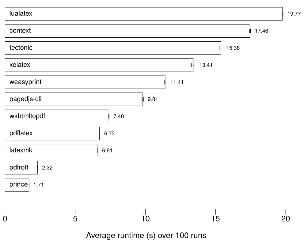
Benchmarked pandoc PDF engines (lower is better)
The LaTeX engines are extremely slow, and this came as no surprise to me. At the end of writing my Master’s thesis, I was often waiting over a minute for XeLaTeX to compile my document with its multiple figures and musical examples. It may look extremely beautiful, but it takes a long time to iterate the feedback (or “edit–compile”) loop. This is the same with programming: if your compiler is slow then it usually does not matter how optimised its output is, the slow compiler is wasting valuable programmer cycles rather than cheap CPU cycles. I believe also that a slow feedback loop hinders flow state, as every time you’re waiting for the program/document to compile, you lose a little bit of concentration. It is for this same reason that I cannot stand doing web design using a framework where I cannot see the results of my changes almost instantly. If I have to wait more than five seconds to see the results of my slight change in padding, then I become frustrated with the process.
The HTML engines are, once again, of varying speed. Prince is by far the fastest, but groff comes in a close second, with a much better quality. Groff is notable, too, for its output size:
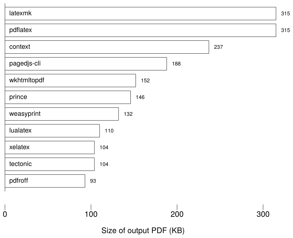
Pandoc PDF engine output sizes (lower is better)
I believe this is largely due to the fact that groff in my case embedded only four fonts in its output PDF, whereas the LaTeX engines embedded up to twelve. I would think therefore that the size advantage for groff would diminish on longer, larger files. For me, the Markdown engine of choice is pdfroff.
Greater things
Using groff as my preferred backend for converting Markdown to PDF piqued my interest in the system, and soon I found the macro set called “Mom” that applies numerous quality–of–life changes and sensible defaults to groff. Mom has a good set of documentation,[7] and it didn’t take me long to begin writing documents using the macro set. I had no idea that groff could accomplish citations/referencing (using refer), figures (by including PDF images created using Imagemagick), diagrams (using pic), tables (using tbl), graphs (using grap — those benchmark graphs above were created using grap), tables of contents, cover pages! Not only is groff quick to compile, but also quick to write. Most commands are a period and a few letters on a new line, rather than the complicated brace expressions of LaTeX.
I recently updated my CV (in LaTeX) and the process underscored how much of my typesetting was just “try something and see how it looks”. Not only did this take a long time to refresh using LaTeX, but no matter how I indented the file, I could not make the markup look clean. I realise now how much I am fighting LaTeX whenever I stray from the happy path (that path being almost unilaterally text and equations).
In groff, the typically all–caps commands stick out to me and, just like LaTeX, are generally semantic rather than aesthetic (“create a heading” rather than “create large bold text”). Although I have never used WordPerfect, I am reminded of how people speak of its “Reveal codes” mode in hushed tones. This quick writing works well with my preferred workflow of vim + terminal. I write a Makefile with a “watch” rule that calls Mom’s frontend in a loop with . As soon as I save a file in that directory, the PDF is compiled.
In fact, many of the advantages of using groff are the same as LaTeX, but with the added advantage of speed and simplicity. Just like with LaTeX, you can dive into the code to change a macro but, unlike LaTeX, I have found Mom’s macros fairly understandable and not nested ten layers deep in some ancient package.
Notes on using groff for academic work
I contain my files within a git repository and make use of all the advantages contained therein, particularly stashing changes for later and working on new material in a separate branch.
I use Mom’s macro to keep chapters in separate files, and maintain a “thesis.order” file that describes which files are to be concatenated in what order. The Makefile reads this file and simply ’s the files together, piping into which handles the preprocessing with refer, tbl, grap and pic.
The manpages for the preprocessors are eminently readable, with a strong focus on tutorial rather than simply documentation of “what you should already know”, but I would also recommend:
- Mom’s own documentaton page on refer.
- James and Schaffter’s PDF document, especially for creating internal links.
- Bentley and Kernighan’s paper on grap (warning: Postscript).
- Raymond — Making pictures with GNU pic.
Below a sample of the in–progress PhD. I don’t want laggy Word and inconsistent styling issues. I don’t want KOMA-Script woes and minutes–long compile times. I want something simple that works: groff!
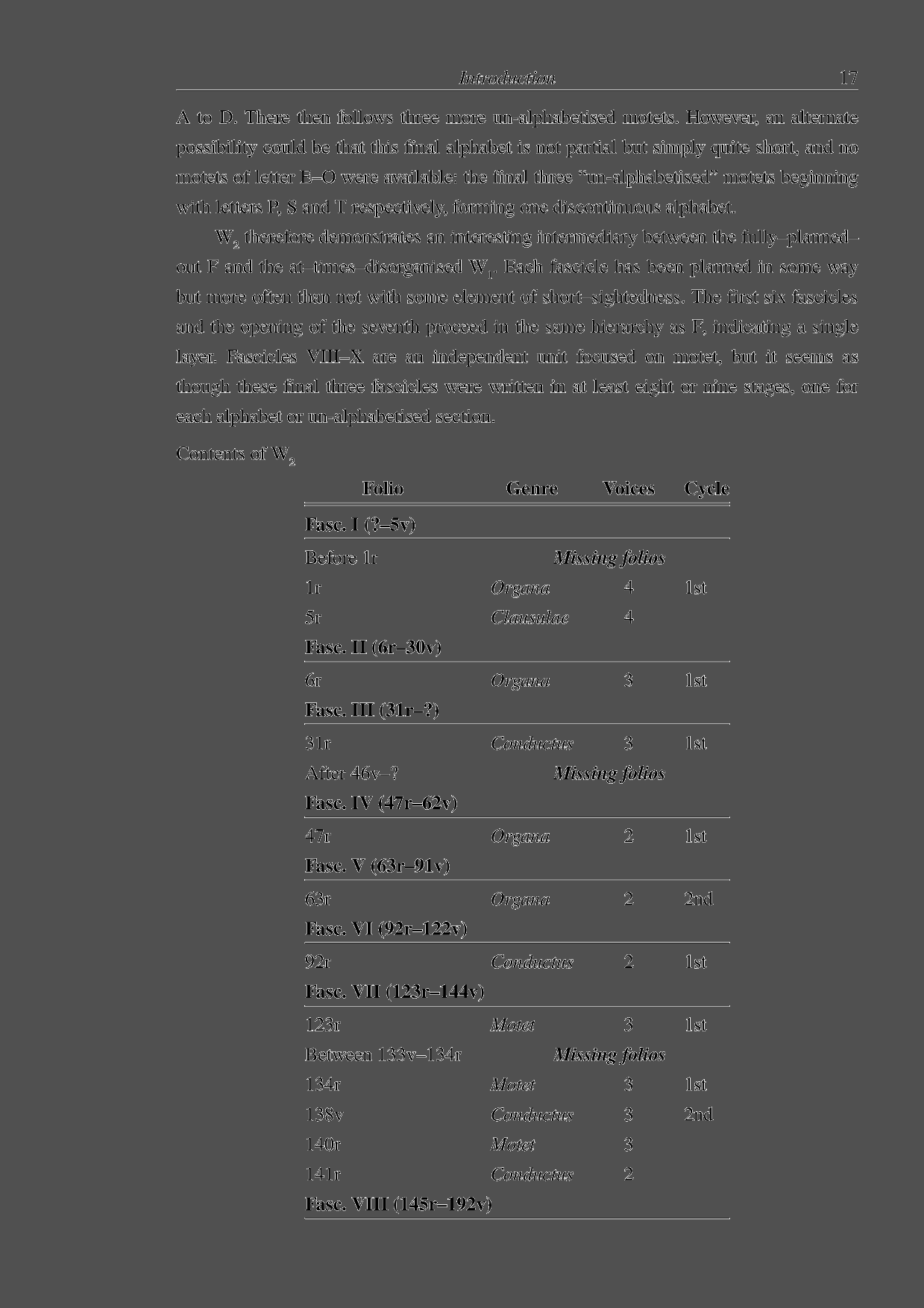
Sample page from groff–powered thesis
- Richard Taruskin, ‘Review: Speed Bumps’, 19th–Century Music vol.29, no.2 (2005), pp.185–295 <https://doi.org/10.1525/ncm.2005.29.2.185> [accessed 21 July 2022] ↩︎
- Nicholas Cook, ‘Alternative Realities: A Reply to Richard Taruskin’, 19th–Century Music vol.30, no.2 (2006), pp.205–208 <https://doi.org/10.1525/ncm.2006.30.2.205> [accessed 21 July 2022] ↩︎
- Harry White, ‘The Rules of Engagement: Richard Taruskin and the History of Western Music’, Journal of the Society for Musicology in Ireland, vol.2 (2006), pp.21–49 <https://www.musicologyireland.com/jsmi/index.php/journal/article/download/12/11/43> [accessed 21 July 2022] ↩︎
- Richard Taruskin, ‘Agents and Causes and Ends, Oh My’, Journal of Musicology, vol.31, no.2 (2014), pp.272–293 <https://doi.org/10.1525/jm.2014.31.2.272> [accessed 21 July 2022] ↩︎
The long slog of inputting both W1 and W2 into CANDR is complete. You can view the result here.[1] F, although its facsimiles have been uploaded to the site, is for now lying with only its system and stave extents partially defined, and work on the tracing–transcription of F is not begun properly. This is simply due to time constraints. Perhaps F, too, will be encoded in the near future. What we do have however, is a database containing the positional data of the musical notation of both W1 and W2. This alone is something that I am proud of (the database file currently weighing in at 231MB),[2] but the most important issue is how to analyse this data in order to extract features that will help me to answer my research questions.
Domains
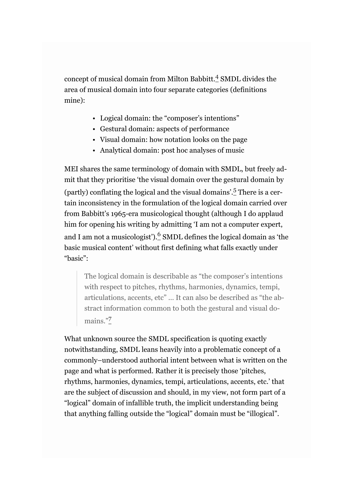
One distinction that I find particularly useful from MEI is that of musical domain. MEI correctly realises that there is no “one encoding to rule them all” and provides tools and schemata for encodings that consider differences of opinion, inconsistencies, and elements of performance practice. MEI accomplishes this through the concept of simultaneous musical domains. MEI acknowledge SMDL (the Standard Music Description Language) as the genesis of this idea,[3] formalising the concept of musical domain from Milton Babbitt.[4] SMDL divides the area of musical domain into four separate categories (definitions mine):
- Logical domain: the “composer’s intentions”
- Gestural domain: aspects of performance
- Visual domain: how notation looks on the page
- Analytical domain: post hoc analyses of music
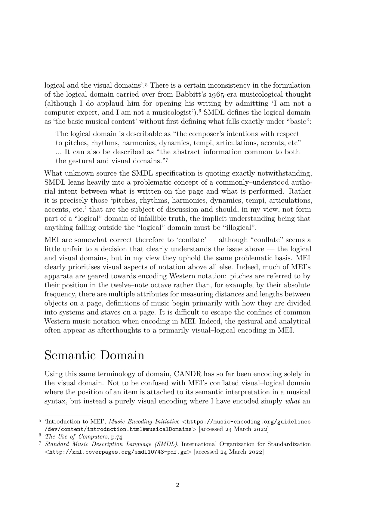
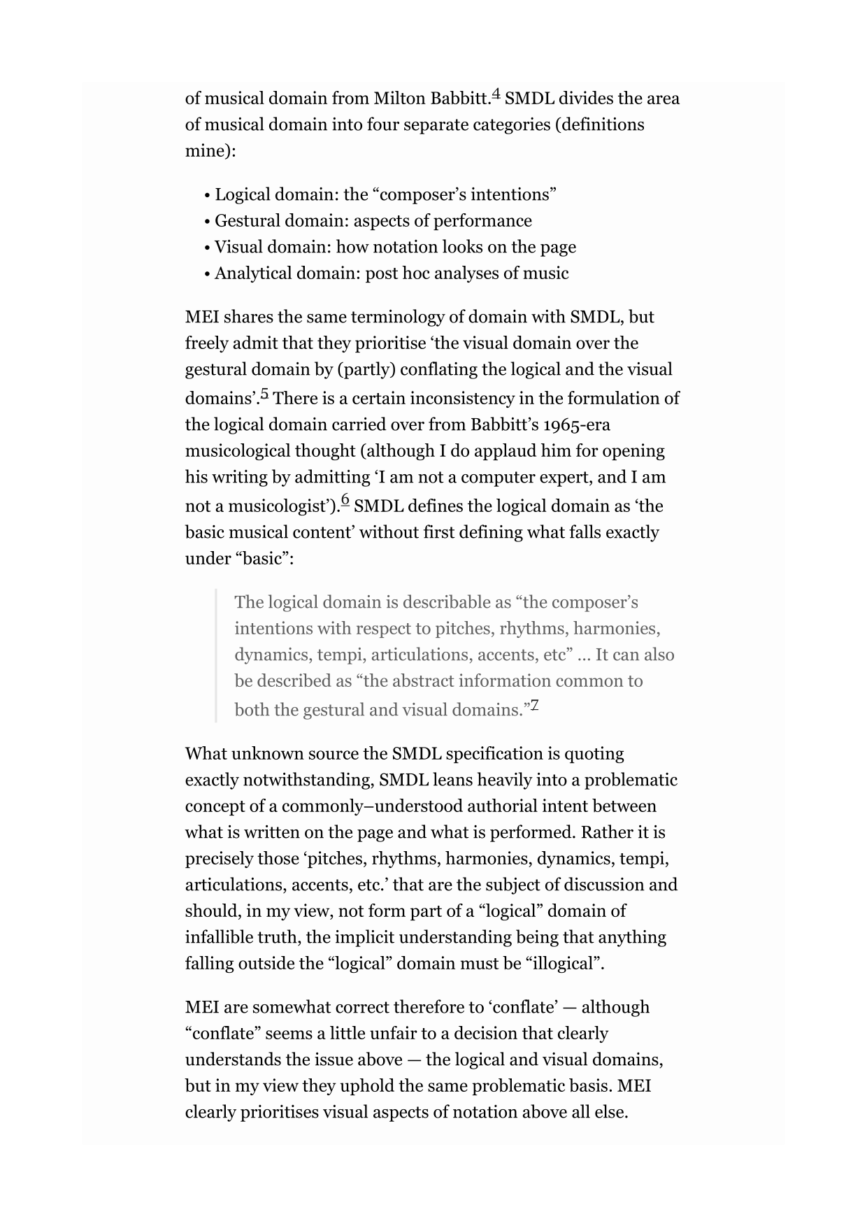
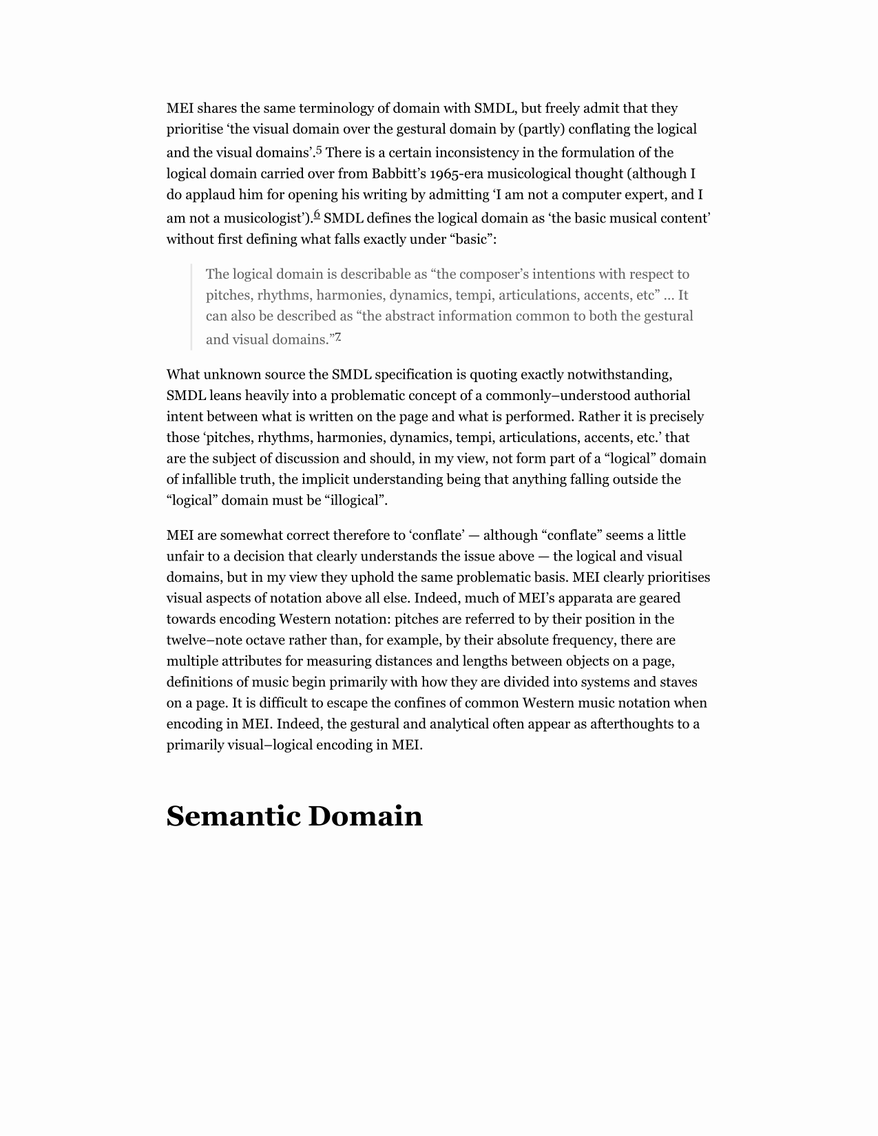
MEI shares the same terminology of domain with SMDL, but freely admit that they prioritise ‘the visual domain over the gestural domain by (partly) conflating the logical and the visual domains’.[5] There is a certain inconsistency in the formulation of the logical domain carried over from Babbitt’s 1965-era musicological thought (although I do applaud him for opening his writing by admitting ‘I am not a computer expert, and I am not a musicologist’).[6] SMDL defines the logical domain as ‘the basic musical content’ without first defining what falls exactly under “basic”:
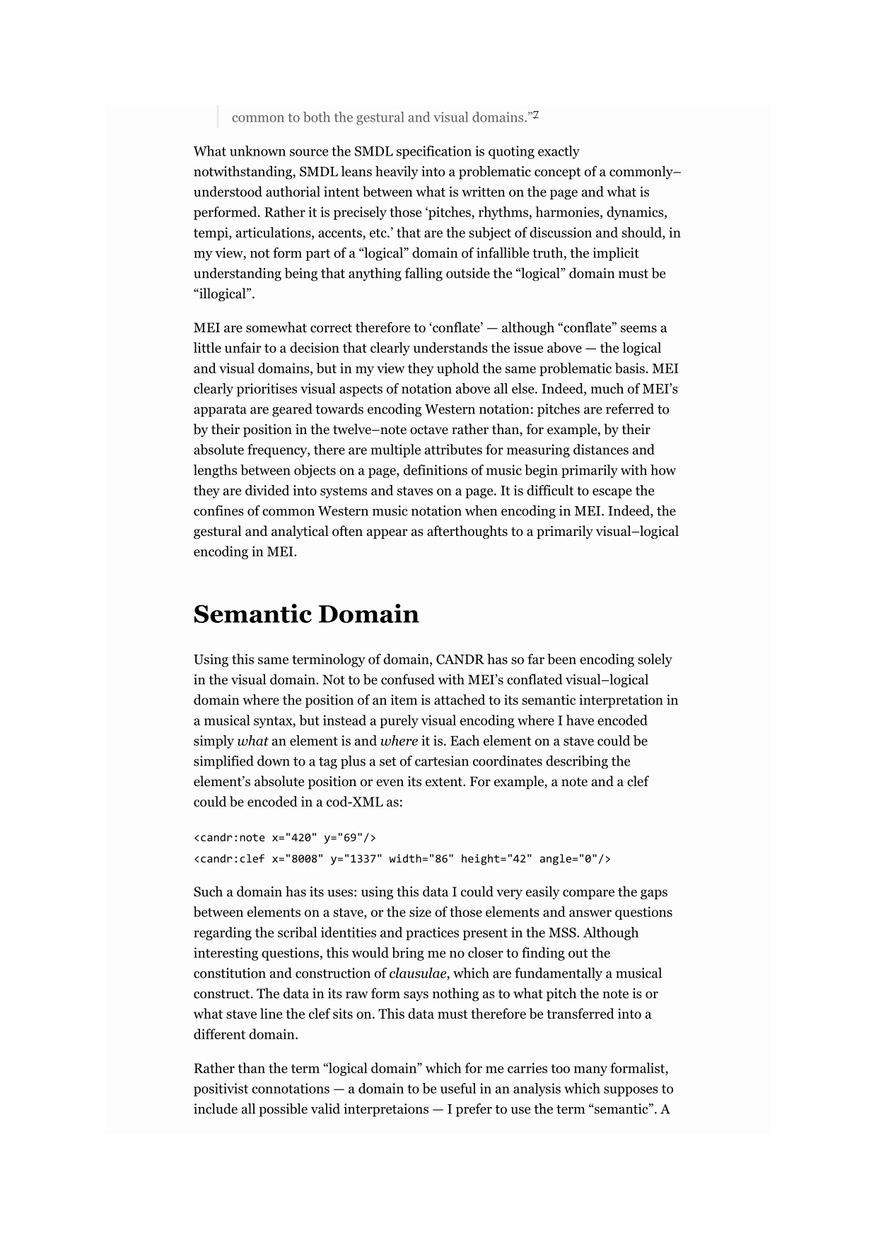
The logical domain is describable as “the composer’s intentions with respect to pitches, rhythms, harmonies, dynamics, tempi, articulations, accents, etc” … It can also be described as “the abstract information common to both the gestural and visual domains.”[7]
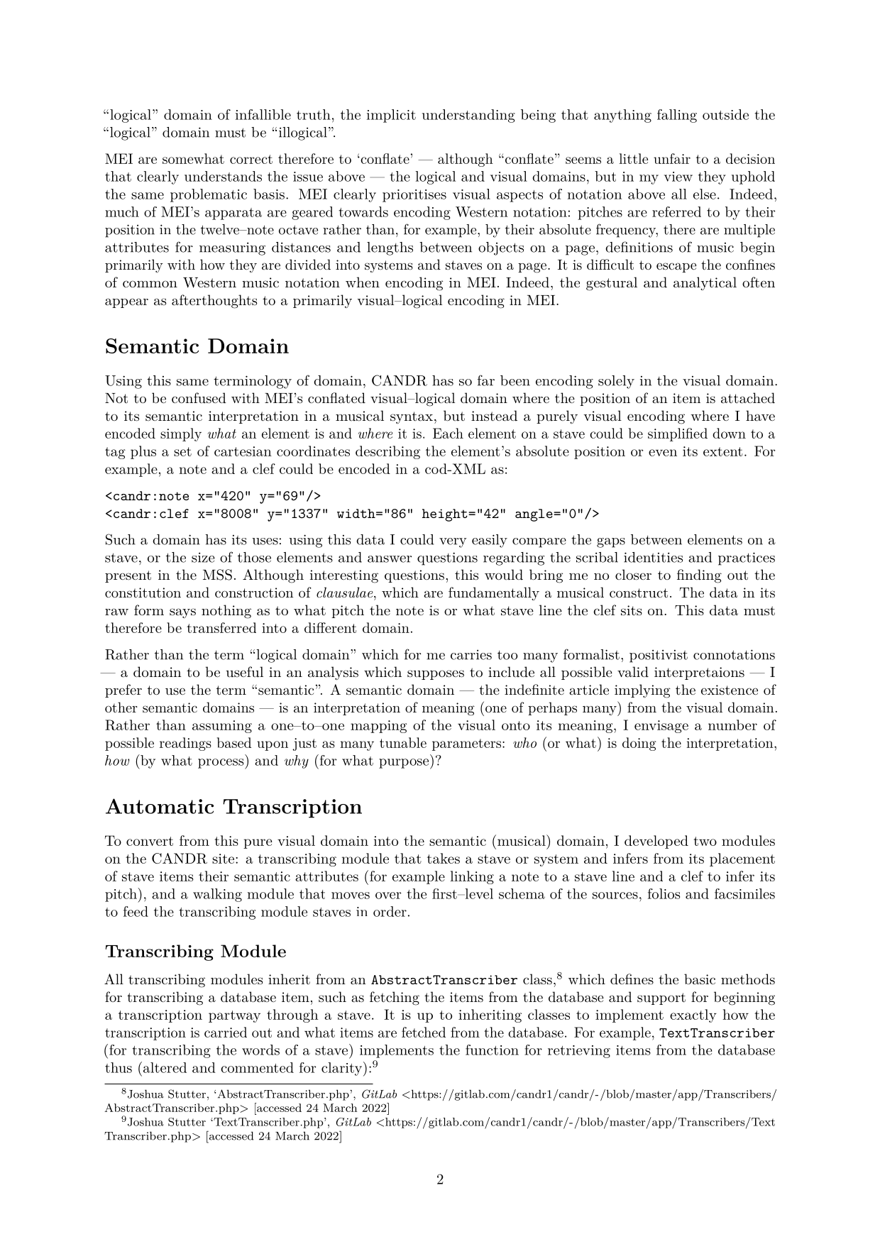
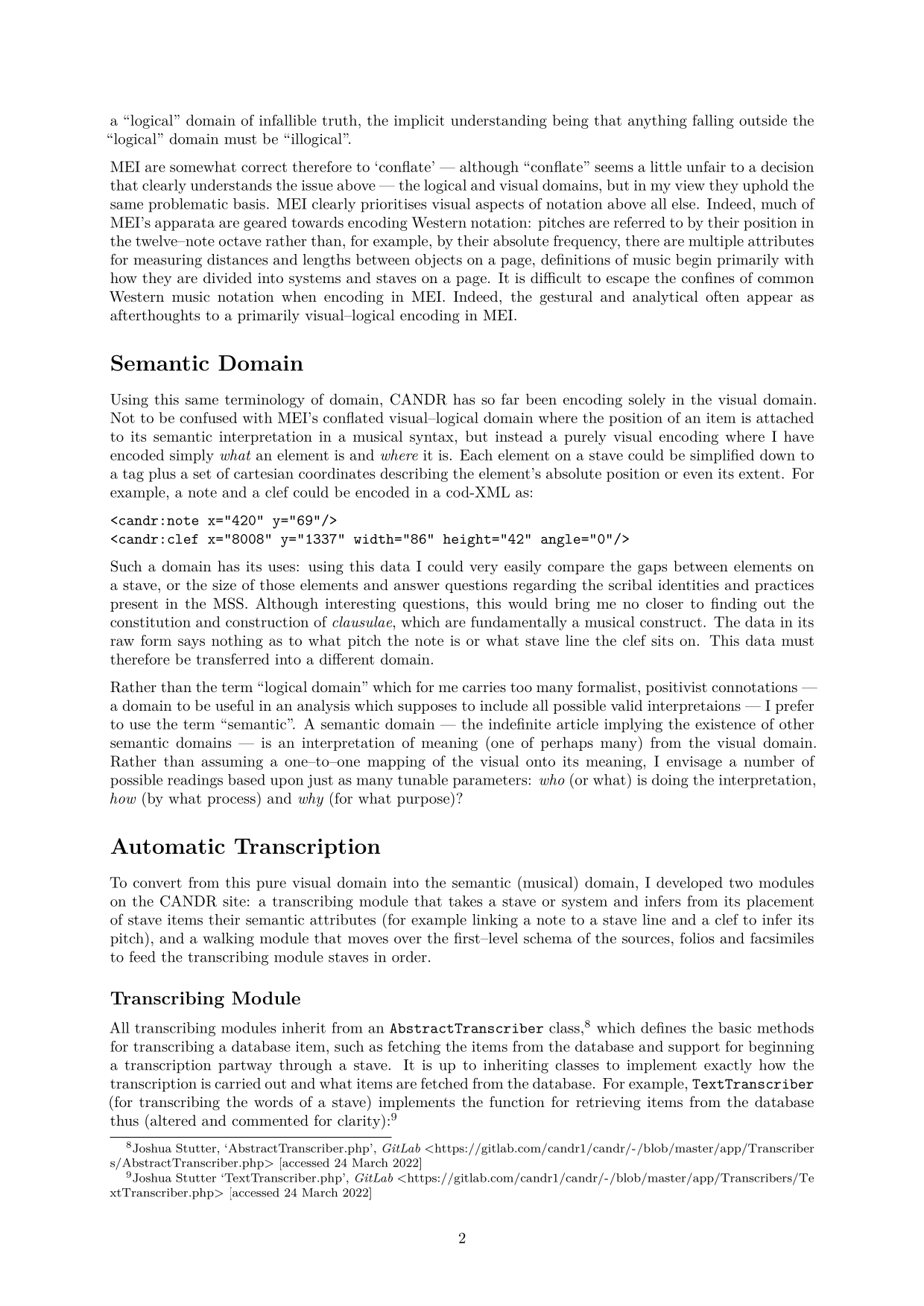
What unknown source the SMDL specification is quoting exactly notwithstanding, SMDL leans heavily into a problematic concept of a commonly–understood authorial intent between what is written on the page and what is performed. Rather it is precisely those ‘pitches, rhythms, harmonies, dynamics, tempi, articulations, accents, etc.’ that are the subject of discussion and should, in my view, not form part of a “logical” domain of infallible truth, the implicit understanding being that anything falling outside the “logical” domain must be “illogical”.
MEI are somewhat correct therefore to ‘conflate’ — although “conflate” seems a little unfair to a decision that clearly understands the issue above — the logical and visual domains, but in my view they uphold the same problematic basis. MEI clearly prioritises visual aspects of notation above all else. Indeed, much of MEI’s apparata are geared towards encoding Western notation: pitches are referred to by their position in the twelve–note octave rather than, for example, by their absolute frequency, there are multiple attributes for measuring distances and lengths between objects on a page, definitions of music begin primarily with how they are divided into systems and staves on a page. It is difficult to escape the confines of common Western music notation when encoding in MEI. Indeed, the gestural and analytical often appear as afterthoughts to a primarily visual–logical encoding in MEI.
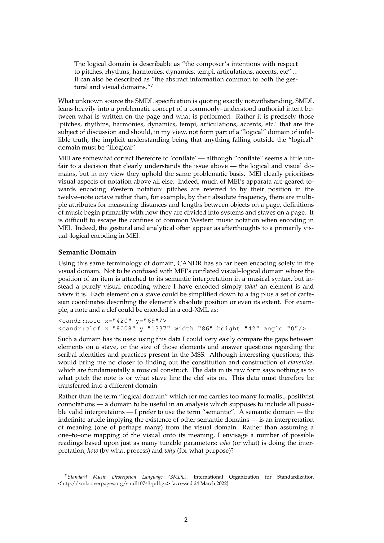
Semantic Domain
Using this same terminology of domain, CANDR has so far been encoding solely in the visual domain. Not to be confused with MEI’s conflated visual–logical domain where the position of an item is attached to its semantic interpretation in a musical syntax, but instead a purely visual encoding where I have encoded simply what an element is and where it is. Each element on a stave could be simplified down to a tag plus a set of cartesian coordinates describing the element’s absolute position or even its extent. For example, a note and a clef could be encoded in a cod-XML as:
Such a domain has its uses: using this data I could very easily compare the gaps between elements on a stave, or the size of those elements and answer questions regarding the scribal identities and practices present in the MSS. Although interesting questions, this would bring me no closer to finding out the constitution and construction of clausulae, which are fundamentally a musical construct. The data in its raw form says nothing as to what pitch the note is or what stave line the clef sits on. This data must therefore be transferred into a different domain.
Rather than the term “logical domain” which for me carries too many formalist, positivist connotations — a domain to be useful in an analysis which supposes to include all possible valid interpretaions — I prefer to use the term “semantic”. A semantic domain — the indefinite article implying the existence of other semantic domains — is an interpretation of meaning (one of perhaps many) from the visual domain. Rather than assuming a one–to–one mapping of the visual onto its meaning, I envisage a number of possible readings based upon just as many tunable parameters: who (or what) is doing the interpretation, how (by what process) and why (for what purpose)?
Automatic Transcription
To convert from this pure visual domain into the semantic (musical) domain, I developed two modules on the CANDR site: a transcribing module that takes a stave or system and infers from its placement of stave items their semantic attributes (for example linking a note to a stave line and a clef to infer its pitch), and a walking module that moves over the first–level schema of the sources, folios and facsimiles to feed the transcribing module staves in order.
Transcribing Module
All transcribing modules inherit from an class,[8] which defines the basic methods for transcribing a database item, such as fetching the items from the database and support for beginning a transcription partway through a stave. It is up to inheriting classes to implement exactly how the transcription is carried out and what items are fetched from the database. For example, (for transcribing the words of a stave) implements the function for retrieving items from the database thus (altered and commented for clarity):[9]
In essence, this function not only retrieves the stave’s syllables from the database, but also ensures that they occur at the right place to be included in a synchronisation link by moving them just right of the nearest note, and sorts them left to right to be transcribed. is a small proof–of–concept for the transcription element, but CANDR also includes an implementation following the same principles. To transcribe music rather than syllables is more complex, but returns MEI (in a CANDR–specific dialect) for a system of music (the limits of which will be discussed later).
Walking Module
Similarly, all walking modules inherit from an class,[10] whose main function begins at any point in a source and walks forward, calling the transcriber, until it reaches any one of many “stop” elements, passed in as an array. For example, given a stave with two elements, respectively listed as “start” and “stop”, the walker will call the transcriber once on that stave with those parameters. However, if the “stop” elements are on another stave, then the walker will call itself recursively on the element above: walking on a stave without raising a “stop” signal will cause the walker to then find the common system and transcribe the next stave in that system. If the “stop” is not found there either, it will go up to the facsimile or even folio level and keep transcribing until that “stop” element is found. The simply has to instantiate a as its transcribing class, and transcribe only the lowest stave (where the words are found) in a system.[11] Once again, there is an for creating MEI documents.[12]

How a walking module walks between first–level schema items
Result
These two elements combine to create automatic transcriptions of the sources into words and MEI. For example, navigating to https://candr.tk/browse/facsimile/86/ will show you the facsimile of folio 43v in W2. If you alter that address to https://candr.tk/browse/facsimile/86/text/, then it will display the transcribed text for that facsimile “regina tu laquei tu doloris medicina fons olei uas honoris Tu uulneris medelam reperis egris efficeris oleum unctionis Post ueteris quem”. Requesting https://candr.tk/browse/facsimile/86/mei/ will yield an MEI document of the music on that page.
Behind the scenes, there is a fair amount of caching to speed up this process. Every time a transcription is requested, CANDR first checks a cache record in the database. If there is a cache hit then it simply returns that cache record. This means that requesting the same transcription twice should not re-transcribe the item, needlessly hitting the database, but returns a pre-computed record. However, if a database element is altered after a transcription is cached then the transcription may be invalid. CANDR notifies all the records that use that element that their transcription may now be invalidated. For example, if a stave has been altered then that change is propagated throughout the cache system: caches for its stave, facsimile and folio are instantly deleted such that the next time the facsimile transcription is retrieved, it must be re-transcribed using the most up–to–date information. This way we can ensure that the caches are never out of date.
The “Setting”
Considering once again the musical domains of the visual vs the semantic, the transcriptions created so far have themselves considered only the visual aspects of the source. We can transcribe staves, systems, facsimile and folios but, more often than not, music flows from one system to the next and from one folio to another. We cannot simply conceive of a source as a disparate set of codicological items, but as a book intended to be read from one opening to the next. The concept of the walker allows for this movement between codicological items as previously described, but it needs to know where to start and stop. How do we find elements to begin and end our transcription? I would like to introduce another concept into this ontology: that of the musical “setting”.
A setting is a semantic rather than visual construct, but relies on visual cues supplied by an editor (completed during the data input stage). I have previously mentioned my concept of the synchronisation link which indicates that two elements on adjacent staves occur simultaneously with one another. The beginning of a piece of music links items from all staves together, and this special kind of link is tagged as being a “setting”. Using these tags, a walker can walk from one tag to the next, returning the music of a setting.
However, these are also tagged and titled by hand, being an editorial creation. It is here that CANDR shades into replication of some of the functionality of DIAMM. DIAMM lists the contents of W1 as a hand–curated inventory (human mistakes included!), listing “compositions” with their titles, “composers” (nearly all of whom are anonymous) and start/stop folios.[13] However, DIAMM considers pieces such as Alleluya. Nativitas gloriose as single items, whereas I treat them as separate alleluia and verse settings. Regardless, these settings can be categorised and listed in CANDR at https://www.candr.tk/browse/setting/. The advantage that CANDR brings is the possibility of then browsing the facsimiles for that setting, and viewing a transcription of the words and music, all the way to the granularity of each note.
This is the effective completion of the online database stage of CANDR. The next analytical stages are completed offline by scraping data from the site.
Encoding Encapsulation
MEI is a hierarchical encoding, by virtue of its tree–based XML format. An MEI document (after header and boilerplate) begins with a base music element, such as and then moves into that music’s components in a divide–and–conquer strategy until it reaches a level where atomic elements can be encoded directly without any children. Looking at MEI’s example encoding of Aguardo’s Walzer from the MEI sample encodings repository, lines 227–254 begin the encoding proper by limiting the initial scope until we reach the first moment of the first stave, a quaver rest.[14] Greatly simplifying those lines to just contain the initial rest, we get a tree structure:
This XML structure can also be visualised as a series of concentric boxes, similar to the CSS box model:

This blog post is full of pretty pictures
Each element can only be linked to other elements in three, mutually exclusive ways:
- Parent: the containing box of an element
- Children: the boxes contained within this element
- Siblings: other boxes that share the same parent element
The in this example has one parent , one sibling and five children: as well as others. These limits are often powerful, as they enforce a strict design philosophy on a document such as MEI. Elements are contained within other elements such that an element can only have one parent. For example, a can only occur in one at a time. This makes parsing and analysing this data structure (a tree) simple as it is guaranteed to be acyclic (i.e. when descending the structure it is impossible to visit an element twice).
Generally this works well for MEI as it is easy to conceive of musical structure as such: rests in layers in staves in measures in sections in scores in divisions in a musical body, and this does work well for for elements that occupy a single space in time, such as simple notes. On the whole it echoes how common practice Western music notation is the de facto standard for encoding and how music must be fit into its confines: for example notes are contained within measures and cannot simply overflow a bar.
How, then, might we encode Notre Dame notation using such a model? Before thinking of MEI exactly, let us consider it simply as a series of boxes. It is simple to draw boxes around a system and its staves and also around smaller items such as notes and ligatures, but in the midground we come across a thorny issue: do we first divide a system into its constituent staves or into a series of virtual timeseries boxes (which we could errantly name “ordines”)? Each has its advantages and disadvantages, and the issue is roughly analogous to MusicXML’s two encodings: timewise and partwise, either encoding measures of music at–once or encoding entire parts or voices at–once. MEI is always equivalent to MusicXML’s partwise encoding.
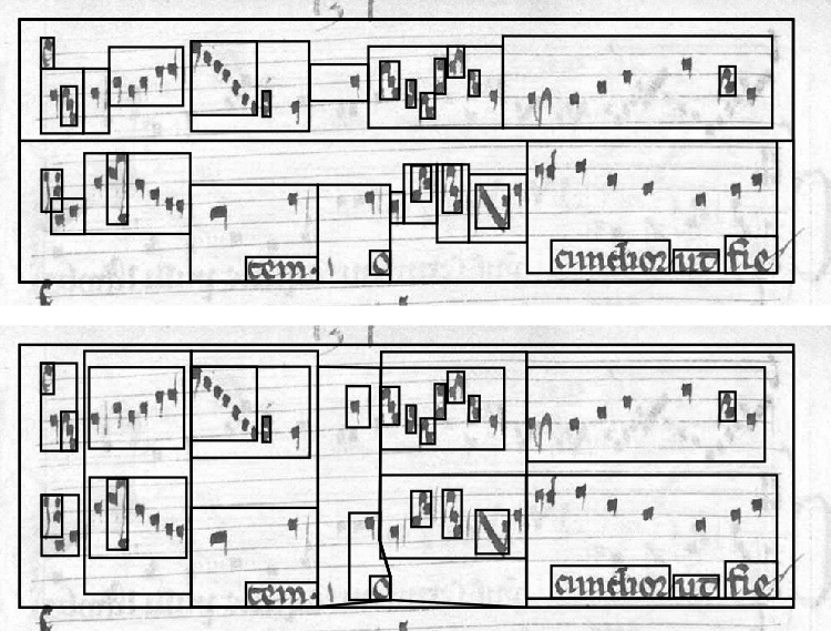
Two attempts to draw boxes around elements: top is partwise (staves first) and bottom is timewise (“ordines” first)

The above conceptualised as concentric boxes
Partwise
- Advantages:
- Each part element is a sibling of its successor and predecessor.
- Staves can be considered at–once.
- Mirrors the exact lack of verticality in the notation.
- Disadvantages:
- The information of which items occur simultaneously is lost. In common MEI or MusicXML, this can be inferred by counting durations, but in Notre Dame notation, rhythm is subjective and up to interpretation. We cannot rely on duration counting.
- Virtual items, such as the idea of a common tactus between parts, or a common ordo length, is also lost.
Timewise
- Advantages:
- Everything that occurs together is grouped together.
- Polyphony can be easily extracted
- Disadvantages:
- Often to reach the next note in a stave, we have to traverse up the structure to reach a common ancestor.
- Infers an editorial synchronisation between parts as a first–class element.
- Cannot infer verticality between a subset of parts.
MEI’s solution to this is to keep the music encoded partwise, but use a attribute to break the encapsulation and link between other items in the document.[15] I use this exact solution to encode Notre Dame music in MEI, but the data model is still unsatisfactory. There is a false idea of musical encapsulation with virtual objects (such as ordines) which is then arbitrarily broken to make connections that are not formalised in the model. This also makes parsing the data much more difficult: more than simply viewing a node and the limited relationships between parents, siblings and children, a parser must now look at the node’s attributes and other objects in the tree, potentially creating cycles. In short, it seems like a bit of a hack. In terms of the structure, what happens if an element has two parents? In which “box” should it belong?[16]

How I link Notre Dame notation together using the synch attribute in MEI
A third way: graph(-wise?)
In fact, MEI provides a whole selection of attributes in the class to indicate relationships between items this way, such as and for temporal relationships. However, these still must be structured in the element. Rather than encapsulation, this music that falls outside common Western music boxes would be better encoded with links between items being first class, in order words encoded entirely as linked data as a directed graph. These kinds of graphs are not of the bar, line, pie, scatter ilk but rather those of graph theory, what we might commonly term networks. Instead of items preceding each other being known by the order of siblings, and items in ligature being known by being children of a “ligature” element, each element would link from one to the next, and an element in a ligature would have a link signifying membership of a ligature. Synchronisation links are therefore simply another link of the same class as temporal relationships or ligature membership.
We could for instance model this as RDF data. Consider the same music as linked data (in Turtle format, using example namespaces for simplicity):
This is a big leap, and understandably much more difficult to conceptualise than the box model, so it can be visualised as an extraordinarily complex digraph (using https://www.ldf.fi/service/rdf-grapher for visualisation):
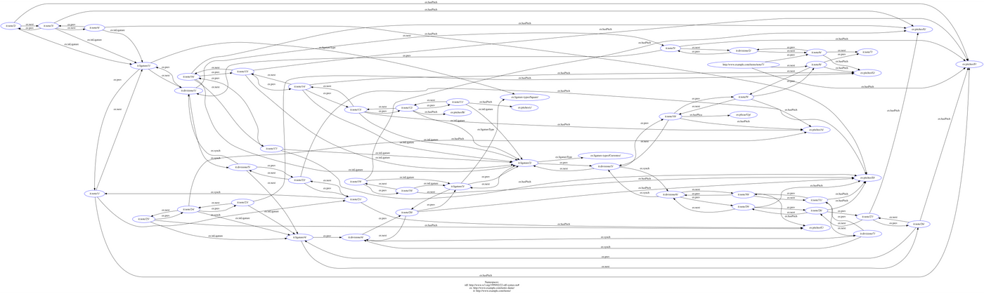
Very large image, zoom in or open image in new tab for detail
To understand this better, let’s look at the node “note/1/” (it is on the centre–left of the visualisation). It has three links going out and two coming in.
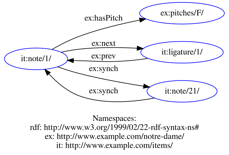
The first, indicates that this note has a pitch of F. It then has two links, one going out and one coming in , indicating that the note’s next item is “ligature/1/”. “ligature/1/” also has a link indicating that its previous item is “note/1/”. Finally, “note/1/” is linked using with “note/21/” in both directions, indicating that these two items occur simultaneously. This is true throughout the graph (although the visualisation tool struggles with the amount of links), so that we can model the data consistently without needing to place the items in boxes (encapsulation). Traversal of this data structure is much more simple, all that we need to do is to examine an item’s links to see how it relates to other items. For example, we could find all the notes with pitch F by examing the “ex:pitches/F/” node and following the links backward (backtracking).
We can use this graph structure (although not in RDF for reasons I will explain later) to analyse the same music.
Creating an Analysis Package
Candr-analysis is a Python package for analysing a Notre Dame notation corpus (although it could be further generalised to more notational forms).[17] It consists of multiple modules that can be linked together to: fetch information (such as from the CANDR site), parse notation, convert a tree–based representation into a graph, transform that graph into subgraphs, link elements in graphs together, and generate analyses based upon those graphs.
Pipeline
Candr-analysis is based upon a data pipeline architecture, where analysis modules are linked together to asynchronously pass data from one stage to the next. The act of creating an analysis is to link pipeline modules together so that the output from one feeds the input of the next.
The root of this is the class, which receives s (or rather objects that inherit from ) and links them together.[18] Once all the objects have been added to the pipeline, then the pipeline is instructed to begin running and wait for the objects to run. Each object runs in its own process, so a resource–intensive component such as graph creation does not necessarily slow down another component such as parsing. This makes creating new analyses simple. For example, an initial stage of text analysis is to fetch all the text transcriptions from the CANDR site. This is achieved by simply running this small script:
It is clear to see from this fully–functional program that it accomplishes three tasks:
- Setting up a pipeline;
- Adding the components of the website scraper, transcriber and a component that saves the result to disk;
- Running the pipeline and waiting for it to finish.
Pipelines of any complexity can be set up this way which allows for a dynamic iteration of analysis ideas, and the ability to save results to disk at any stage allows for analyses to be created, saved, resumed, re-run, and meta-analyses to be created.
PipeObjects
Adding new functionality to Candr-analysis is as simple as inheriting from the base class of and defining a generator function to take in an input and returning sets of output to be passed to the next object in the pipeline. Below are some objects that I have already created for my uses:
Scraping
A “scraping” is one that views a data source, such as the CANDR site, and generates metadata based upon that source. For example, the scraper views the setting list page and uses its RDF markup to create a rich list of settings in the sources.
Transcribing
A “transcribing” takes a single data endpoint and fetches an individual transcripton of that point. For example, the transcriber receives a CANDR endpoint object and fetches its respective text transcription. Similarly the transcriber fetches the MEI transcription.
Parsing
A “parsing” takes an unparsed input, such as one from the CANDR site, and parses it into something more useful for further analysis. There can be more than one parser for any input, for example a parser may only be interested in certain subsets of the data. Text generally needs no parser, but the MEI parser validates and transforms an MEI file into a graph–based representation as outline above. The MEI parser defines multiple relationships (edge types in a multi–digraph, roughly analogous to the data model of RDF) between items. These have been generalised so that they could be used with any repertory of music, not just Notre Dame notation, and the graph can support more kinds of links:
- Sequential: B follows A
- Synchronous (Hardsynch): A and B occur at the same time
- Softsynch: A and B are some distance away, but their distance can be computed, the weight of this edge being defined as the reciprocal of the distance between the nodes.
Transforming
A “transforming” performs some sort of transformation on parsed data before it is analysed. For example, data may need to be weighted correctly or converted from one data structure to another.
Analysing
An “analysing” takes a corpus of data and performs some analysis on it, generating some new artefact — typically a database — that can then be interpreted.
Interpreting
An “interpreting” extracts useful information from an analysis. What that information is depends greatly on the type of analysis being done.
Utilities
A utility is some quality–of–life object that can help make the workflow simpler. For example, I have found that a good workflow is to scrape and transcribe in one step, taking all the necessary data from the network in one go before moving onto following stages. The code above uses an object that dumps its input directly to disk, and there is another object that can read data from disk and send it into a new pipe. Examining these intermediary files is also indispensable in debugging.
Graph Analysis
What remains, then, is the analysis of these graphs. Although the narrative inroad to Notre Dame notation as a graph was through RDF, Candr-analysis internally uses the more general–purpose library NetworkX to generate its graphs during parsing,[19] and SQLAlchemy for on–disk graphs.[20] The reason for this is that although RDF’s model fits my data model and is simple to comprehend, it is designed for linking humanistic data using strings. There is therefore no RDF implementation efficient enough for this use case. For example, I could use SPARQL to query an RDF store for this dataset, but the number of nodes that will be created and the density of connections between the nodes would likely be far too much for a sensible RDF implementation to handle.[21]
N-grams
A common methodology in computational linguistics is that analysing a text’s n-grams, splitting texts into tokens then combining sequential tokens of size n. In other words, creating 2-grams (bigrams) of “the cat sat on the mat” would yield the following set: “the cat”, “cat sat”, “sat on”, “on the”, “the mat”. 3-grams (trigrams) of the same text would be “the cat sat”, “cat sat on”, “sat on the”, “on the mat”. These can be used to detect similarities and syntax between texts other than simply counting word occurrences (which would be 1-grams or unigrams). N-grams can also detect word sequences and context. Generating n-grams for CANDR text transcriptions is as simple as defining a that returns n-grams for input strings:
However, the more difficult task is that of generating n-grams of music as this is a problem that has not yet been solved, indeed n-grams generally cannot be generated for more than single streams of data. Monophonic music (such as chant) could simply be tokenised into its constituent pitches, but polyphonic music (such as the Notre Dame repertory) depends not simply on what pitches occur in what order, but also what is happening in other voices at the same time. I propose a method of extracting workable n-grams that are not represented by tokens but by graphs, and maintain their synchronisation contexts to then be analysed as a whole corpus graph.
Consider the same passage of music we looked at previously. We could more simply represent it as a graph like so:
Simplified graph of music
In the upper voice, there are four notes in the first ordo: F, F, E, D. In the lower voice, there are only two: C, D. Not everything is synched together — only the initial F to the initial C — so we don’t know exactly where the D comes in the lower voice. We must therefore make some assumptions. Since there are half as many notes, we can assume that in this voice the notes move at roughly half the speed as the upper voice. The C in the lower voice must change to a D somewhere around the E in the upper voice. This is likely incorrect, but over the course of millions of grams, these assumptions should average out.
If we wanted to created unigrams of the first ordo, we could create:
F→C
F→C
E→D
D→D
The next ordo (with only one note in the lower voice) would all be paired with F:
|→|
F→F
G→F
F→F
G→F
A→F
A^→F
And so on. However, if we wanted to create bigrams, we could move with the same ratio, but using pairs of notes. In the first ordo top voice, there are three bigrams: FF, FE, ED. The lower voice only has one bigram: CD. Our graph bigrams are therefore:
FF→CD
FE→CD
ED→CD
There are no trigrams, so we must overflow into the next ordo to create one:
FFE→CDF
FED→CDF
EDF→CDF
DFG→CDF
By using the graph representation of the music, these n-grams cannot be confused with other n-grams with other synchronisation patterns. This is because there are also soft synchronisation (softsynch) links computed between elements of the graph. Consider this polyphonic music:
A simple contrived example
This yields four bigrams: FF→C, FE→C, EF→C, FE→C. There is a duplicate bigram, FE→C and this might incorrectly indicate that they are identical. The first bigram is closer to its synchronisation C than the second and this should be reflected in its n-gram. To solve this, the softsynchs are computed such that every note is linked to every other by the reciprocal of its distance (here shown in dashed lines). The first FE→C bigram has softsynchs of .5 and .33 respectively whereas the second has .25 and .2: the synchronisation link between the voices in the second is weaker although the pitch content of the bigram is identical.
N-grams in a corpus graph
A n-gram can output subgraphs of a graph of a passage of music as a series of n-grams to then be processed further. In my analysis, the n-grams are further split up into their constituent voices, taking the mean of their synchronisation weights, but split into hard vs soft synchs. For example, the first bigram in the above example, FF→C would yield two records: FF and C. These two records are linked by a hard synch of 1 and a soft synch of 0.5. The next bigram, FE→C links FE and C with a hard synch of 0 and a soft synch of 0.42 (the average of 0.5 and 0.33). These links are also linked back to the “subject” of the link, for example the setting that the n-grams were generated from. This corpus graph is then stored on disk as an SQLite database with millions of connections made between n-grams.
We can query this corpus database by comparing the graph to another piece of music and how similar it is to edges in the graph. For example, another piece of music may contain FE→A. This would match FE, but in our graph there is only FE→C. A scoring function controls the weight of certain parameters in calculating which grams more closely match the queried grams. We can tweak parameters of the graph search to control for gram size, the strength of hard vs soft synchs and “wrong synchs” such as the example just mentioned where there is a synch from FE but to C rather than A.
By way of example, we could give hard synchs (which always have an edge weight of 1) a scoring ratio of 10, and soft synchs a weight of 5. Wrong synchs are weighted less, say 0.1. We calculate the difference between the bigrams as:
Where Hw is the hard synch weight, Hr is the hard synch ratio, Sw is the soft synch weight and Sr is the soft synch ratio. Let us imagine that we query the graph with FE→C with a hard synch of 1 and a soft synch of 0.5. This would match the first bigram more than the second as the score for the first bigram would be:
Whereas the second bigram’s score would be:
However, if we query FE→A with a soft synch mean of 0.64, then this would score 0 on hard and soft synch, but if we calculate hard and soft synchs again with the wrong synch and multiply by 0.1 to find the score:
We repeat this calculation for all the grams in the queried music and keep a cumulative score of subjects (such as settings). Subjects that score small differences over many grams may be inferred to be similar to the queried music. The overall idea of this analysis is not to generate a single, binary truth “X is the same music as Y”, but a view on a repertory (I can see this methodology generalised to other repertories of music) where, given certain parameters and a particular viewpoint, two pieces of music display a high degree of concordance saying some more along the lines of “X, when split into bigrams and weighted using these synch parameters, is most similar to Y but also scores highly on Z etc.”
- This same breaking of encapsulation is found in how MEI must deal with ties and slurs, although they use another weird attribute hack: https://music-encoding.org/guidelines/v4/content/cmn.html#cmnSlurTies ↩︎
- Joshua Stutter, ‘pipeline.py’, GitLab <https://gitlab.com/candr1/candr-analysis/-/blob/424a2b0162b8f4055f35dc387ce6638b2dea4add/src/candr_analysis/utilities/pipeline.py#L128> [accessed 24 March 2022] ↩︎
To cut a long story short, I had vastly miscalculated the costs for using the ✨ magic ✨ of Google, and they were going to send me a bill for £200. Panic, delete account, please don’t charge me, I can’t afford that. Well, that was a bit of a dead end, but I’m a lot wiser now (see last post). The “RightWay” can be a productive way of working, if you have a budget and a whole team of people to support. I have neither, so I returned to the world of the pragmatic, and spent a few days migrating everything off Google and to Mythic Beasts, an independent provider based in Cambridge with a fantastic name, which I have used before.[1] They charge me a few quid for the pleasure, which is a small expense I am happy to deal with! Nothing is as magic or as new, my efforts to automate everything have been practically for nought, and I will have to do the ML myself on my own computer, but at least it works.
Better ML
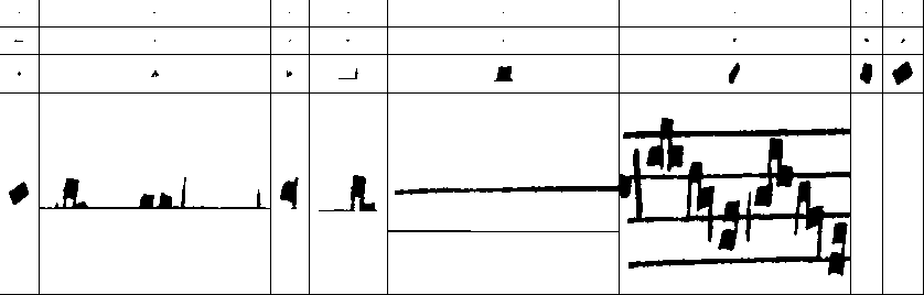
CANDR now has a temporary domain name: www.candr.tk, where I have begun to input some of W2 to test the ML.[2] More tweaking and cleaning up of the ML code has improved the accuracy a surprising amount. The boring detail is to do with weighting. Take, for example, the notes. I preprocess the data by (basically) making two images. Image one (the input) is the original stave, and image two (the output) is blank with the features I wish to detect marked up (it is a little more complex than this, I’m not using pretty colours). Put simply, the training phase of the ML takes both images and attempts to alter its neural network to best recreate the output from the input.
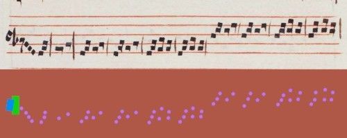
The original stave against a pretty representation of the output
As you can see from the image, in this case there are many more times blank “nothing” spaces than useful features, so the ML frequently got away with just predicting nothing for every sample, the important notes and items would not be enough to get it off the ground, so to speak. To counteract this, during my preprocessing, I now count the number of “nothings” and the number of features. Say I have 100x more nothing than feature, I can then pass the inverse of that into the training, such that if the ML predicts a note wrong, it is 100x more likely to effect a change on the neural network than predicting a blank space wrong.
RAM Emergency

I wish. Everyone remembers this episode of *The IT Crowd* for the “street countdown” storyline, but forget Jen’s exclusion from Douglas’ secret workout sessions. A reminder that the writer of *The IT Crowd*, *Father Ted* and *Black Books* is rightfully cancelled and permabanned from Twitter for being transphobic.
Another problem that I have run into is the ever–increasing size of my dataset. My computer has a fair amount of RAM, and the dataset fits easily in that space (currently sitting at around 2GB after preprocessing), however the RAM issue lies in the implementation and what should hopefully be the last of the gory technical detail. The language I am using, Python, is the most popular and supported language for developing high–level ML in, as it is simple and fast to develop in and easy to pick up with few gotchas. However, it gets itself in trouble with extremely large datasets.
Python, like most modern programming languages, is garbage collected, in that every time you make a new variable, it automatically allocates space for that variable but crucially you do not have to tell it when you’ve finished with that memory or manually delete everything as you go along. Every so often, the garbage collector finds all the variables you’re no longer using, and frees that memory back to the operating system. AFAIK, Python’s garbage collector is quite lazy: it doesn’t come round very often and will regularly not actually take the garbage away, thinking that you actually haven’t finished with it, and you’re intending to use it later. Often this is correct, and for small programs it doesn’t matter very much as all the memory is automatically freed when the program finishes. However, for long–running programs (like this one!) we can quickly run out of memory, compounded by another issue called memory fragmentation which I won’t go into.
Under the hood, Python uses the allocator to get memory from the operating system. takes a single argument: how much memory you would like allocated. does not warn the garbage collector that we’re running out of memory, or force it to return memory to the operating system. often will keep allocating memory until something breaks. I believe this was what was occurring with my program. Although the dataset was only 2GB and I have many times that available on my computer, my program was passing through the data multiple times, allocating different copies of the data as it went, fragmenting and duplicating until it ran out of memory. I managed to mitigate this somewhat by manually marking large variable as done with using Python’s , but often they still would not be garbage collected ( is a marker for deletion, not a command to delete-right-this-very-second). This problem was only going to get a thousand times worse when I increase the granularity of the ML, and use more staves as training data. Even if I managed to completely quash the memory fragmentation issue, I anticipate that my dataset will grow large enough not to fit in RAM, even in the best of cases.
I therefore must save my dataset to disk, and access it a bit at a time when training. To do this, instead of saving all the data into one huge variable, I developed a small class (inspired by a popular data science library base class of the same name) that wraps a SQLite database. Instead of keeping the data in memory, before training it is packaged up into batches and saved into the database file. This also has a side effect advantage of forcing the memory to be reorganised contiguously. Each training batch fetches only the next record from the database rather than the entire dataset, and so the size of the dataset should now be limited only by the size of my harddisk. Disk is slow however, many times slower than RAM and it takes upwards of half an hour of crunching to package the data and save it to disk. I really don’t fancy fine tuning it any further, so I now use that dataset as a cache that can be fed back into the training rather than recalculated on each and every run.
Phew! Hopefully that should be the final technical tangle I get myself in.
Putting it all together
There are still some silly little bugs plaguing the transcription interface, the most most notable of which being divisiones that rudely do not delete properly when asked, sudden bouts of unresponsiveness, and plicae being applied to the wrong notes. However, I can work around these, and most importantly I have added a lovely big button to fetch the ML predictions from the database and populate the stave for checking and fixing. Please enjoy this video of me transcribing some staves with the help of ML.
I ramble and transcribe a system.
So how long is this going to take, and is it feasible? At the database prompt, here are two useful commands to give me an idea (comments on the right hand side).
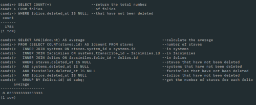
Two database commands to calculate my heuristic.
The first command reveals that there are 1784 folios in the database. My terminology is a little confusing as in the database, folios are defined as manuscript surfaces that are named (n.b. named rather than numbered). For example, “42r” is a different folio to “42v”, even though we would call them the same folio as it has a different name. In practice, folio is better approximated as page rather than folio as one “folio” usually has a single facsimile. This figure of 1784 includes all the facsimile images of F, W1 and W2.
The second command indicates that, of the currently–defined staves, there are on average 8.83 staves per folio. This means 1784 x 8.83 = 15752 staves to transcribe in total. I have transcribed 273 of them in the past week with and without the help of ML. Without ML it takes a gruelling eight minutes per stave to get everything sorted, the majority of the time being taken clicking on all the notes. With ML at its current accuracy, the time is taken down to between two to three minutes per stave. The most successful predictions are staff lines (almost perfect each time) and notes (mostly perfect). This is nearly a threefold improvement and goes to show that this has not all been for nothing!
But can I do it all? Time for a back–of–the–envelope calculation. Here’s the envelope:
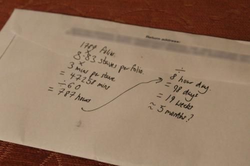
This blog post was delayed because I couldn’t find an envelope for this bit: one of the downsides of going paperless
So, about five months of forty–hour weeks just sitting at the computer pointing and clicking? This is such an interesting figure. It’s neither so small as to be a simple endeavour, like a fortnight, nor so large as to be an unreasonable task, like a year. Likely it would take a little longer due to various issues that will surely crop up, but then again I anticipate that the ML will improve, not by too much as to completely change matters, but small improvements. I think five months is a good estimate.
I could say that it is all too much and I should trim things down, but on the hand the idea of having it all is so inescapably alluring. To be honest I am not sure, with COVID as it is, that I’ll be doing much else this summer, and will probably be stuck inside again anyway (sorry for the downer). Perhaps five months of clicking will be the best use of my time‥?
I have always considered myself further to the right of this image. Nothing that I have ever created has really had that many consequences, so I prefer to “move fast and break things” because my projects have nearly always been for my own benefit. Onoseconds[1] have been entirely my mess to clean up when I completely break my project. I have been influenced in the way I work by Oz Nova’s article You are not Google[2] where he makes the case that it is extremely tempting to over–engineer solutions when the simplest, most pragmatic solution will probably do just fine. It is unlikely you really need that 99.99999% uptime.
This has kept me closer to the laissez–faire attitude, and I have always been sceptical of solutions that will feed two birds with one scone, or even solve all my issues at once! I have found that these solutions will likely bring in more issues that I didn’t have to contend with before, for example instead of just changing one thing I will have to go through a whole process to get the same result (more of that later).
Moving to the left
My last post was very much an example of that (perhaps too wild) attitude. It was definitely more of a proof of concept of using such ML techniques to recognise and locate features on ND polyphony manuscripts. However, the code that got me there was rushed, hacky and buggy. For example, each model was a hacked–together Python script. When I created a new model, I foolishly just copied the script to a new file and changed the bits I needed, rather than abstracting out the common functionality into other bits of program. I had perhaps taken too much to heart that quote “premature optimisation is the root of all evil”.[3] Regardless, those scripts obviously needed cleaning up at some point. The git repositories, too, were a mess (now cleaned up into a different kind of Dockerfile mess).
CANDR as it is, was written in that same vein, but has since been cleaned up. Not as hacky, but written very simply in good ol’ PHP using a thin framework and backed by the disk–based SQLite database. However, when I began to think about how to deploy my machine learning models onto the website, into the cloud (although I detest that expression), my infrastructure must become more complex, and I must move closer to the “Right Way” of doing things.
As the machine learning models are fairly CPU intensive and benefit from being extended by graphics cards (GPUs), it certainly will not do to have them running on the same service as the website frontend. That way, every time the models are trained, the website will crash. Not good. I had to deploy the models onto a different service to the website. However, they also need access to the database, which right now was locked on the hard drive of the website service.
I began therefore by migrating my simple SQLite database to a more flexible but complicated PostgreSQL instance on Google Cloud (not the most ethical cloud provider, but the best of a bad bunch). I went with PostgreSQL as MySQL (the other option) is really quite difficult to work with when you have lots of variable–width text fields.
I eventually landed on an infrastructure which works like so:
Sequence diagram of infrastructure
This began as a simple way to train the models, but through various small necessities has become larger as a move towards the fabled “Right Way” of doing things. This includes modern technologies such as Continuous Integration / Deployment (CI), Docker images and Kubernetes (which I have gone from zero knowledge to a little knowledge on). Simply put:
- CI is a way to make a change to your code and the resulting app or website to be automatically built for you.
- Docker images are pickled versions of services that can be stored as a file, uploaded to a registry and then pulled from that registry and deployed at will.
- Kubernetes is an architecture that can deploy Docker images with zero downtime by maintaining multiple running copies of those services and performing an automatic rolling update of those services. In addition, if you have passwords or secrets that need to be passed to those services, it can inject those at runtime rather than your Docker images being passed around with passwords stored inside.
What I initially wished to occur was that a regular job (say every 24 hours) would spin off and train the machine learning models. However, I soon realised that if I’m provisioning a large, expensive machine to train the models, I can’t have it running all the time wasting money here and there. The machine that serves the website costs only a penny an hour, but a machine powerful enough to train machine learning models costs a pound an hour. I could not leave that machine running, but needed to provision it when necessary, and only when there is new data.
Therefore, I use a level of indirection: a “director” service in CANDR ML Runner[5] provisioned on the same machine as the website. The runner checks the status of the machine learning and is responsible for provisioning the ML service via Kubernetes (i.e. flicking the big switch to turn the expensive computer on). This frees up the website, and all other services can check the runner service to see the status of the ML training. As the runner runs on the same cheap machine as the website, it does not incur any extra cost and updates the predictions only when the training and prediction has been completed. This way, the website can retrieve the most up–to–date predictions from the ML.
Furthermore, the entire build process has been automated using GitLab’s CI. As soon as a change is made to the master branch of the codebase, the website and ML tools are rebuilt automatically and redeployed (again via Kubernetes) to live. This adds another layer of complexity to the diagram above.
It finally works‥ but it is rather reminiscent of this video:
The git repositories that host CANDR are split into two: and .[1] The former hosts the codebase and scripts for CANDR to operate, and the latters stores a dump of the database in a text format (a raw SQL dump) along with the images uploaded to the database as well as the necessary scripts used to transform to and from the database format (SQLite). The project clones both of these repositories and keeps them in separate directories, such that a change in the database does not effect a change in the codebase, and vice versa.
Manual tracing
I’ve been fixing bugs in the frontend of CANDR by uploading sets of facsimiles and attempting to input a few staves here and there, seeing what issues crop up along the way. Exactly as I had hoped, input is relatively fast, such that I can trace the key features of a stave of ND music and save it to the database for processing in under a minute. I am aiming to get a large proportion of the ND repertory traced in this manner to create a large dataset for analysis by next year. I have implemented an automatic guide on the site (the “Transcription Wizard”) that tracks transcription process and automatically leads you through each step of the tracing and transcription process for an entire source of music. The wizard tool takes you through the categorisation of a source to its stave transcription, and each stave is quite simple to transcribe.
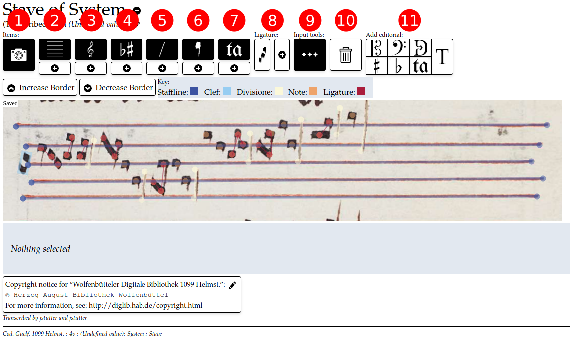
Labelled screenshot of stave editor window: 1. Toggle facsimile visibility 2. Toggle staffline visibility and below, add staffline 3. Clef visibility and add 4. Accidental visibility and add 5. Divisione visibility and add 6. Note visibility and add 7. Syllable visibility and add 8. Tools for adding ligatures and adding notes to ligatures 9. Multi-input tool. When toggled, as soon as an element has been added, automatically adds another of the same type 10. Delete selected element 11. Various tools for adding editorial elements
Using this editor, my personal workflow is thus:
- Trace the stafflines using the staffline tool (2). Use the multi-input function (9) to trace all of these at once. There are typically four to six. It is important to trace these first as they will form the basis for the pitch content of other elements such as clefs, accidentals and notes.
- Trace non-note data. I usually like to begin with the clef (3) as all staves need one of these (existing or editorial), then a starting accidental if present (4), finally using the multi-input tool once again to trace the divisiones (5).
- Trace the notes (6). Use the multi-input tool to click on the note heads, taking care to see which have plicae and which will be transcribed incorrectly by looking at the green staffline outlines.
- Go back over the notes and add plicae and manual shifts where necessary to correct the notes’ transcription.
- Add syllables to notes (if present) making a best guess as to which note this syllable is attached to.
- Finally, use the transcription wizard (not in screenshot) to mark this stave as transcribed.
Once all staves in a system have been traced, you can then use the transcription wizard to mark the system as transcribed, and it will suggest that you add system synchronisation tags to the system. This is a fancy way of saying: add lines between staves that indicate that these events occur simultaneously. A setting of music can then be broken down into “chunks” of polyphony for processing in XML (see previous posts). It will be my aim during analysis to detect which chunks can be grouped together to form clausulae and then how these clausulae are passed around the repertory.
A chunk can be as small or large as you like, but I like to make as little editorial input with regard to inferred rhythm as possible, relying on visual cues to synchronise the staves, such as alignment and the size and shape of divisiones on the page. The scribes of the manuscripts clearly intend some moments to be synchronisation points. For example, it may be possible to imply through rhythmic interpretation that two notes occur simultaneously, but it is more obvious that two divisiones are simultaneous when they are written directly above one another at the end of a system. In this way, it is usually short, synchronous ordines of polyphony that are collected into chunks. Longer, more hocketed passages I will usually shy away from making into smaller chunks as I don’t wish to editorialise a rhythm upon polyphony that is not fully understood. If such hocketed passages are to be passed around in clausulae, then they are likely to be transmitted as single units: half a hocket doesn’t make musical or poetic sense.
Uploading the dataset with some script-fu
In August, I grew bored of just drawing some lines and boxes so decided to source the public domain or permissibly–licensed manuscript images for the three main sources (F, W1 and W2) and upload them in total to the website. The images of these can be downloaded as a large set of numbered JPEGs from the respective library websites, so I had a task at hand to organise these JPEGs and label them, then upload them one–by–one to the website, creating a folio and facsimile record for each, then grouping them all into facsimile sets. As can be seen from the folder of ID-named files in the image store of the data repository, this was a lot of files to upload![2] However, I did not complete this mammoth and repetitive task alone. I wrote two shell scripts ( and ) to streamline the tagging and uploading process of these files.[3]
The JPEGs as I had downloaded them were luckily saved in a numbered order, so moving back and forth through the numbers in an image viewer moved back and forth in the manuscript. By flicking through the manuscripts, I took a note of where the foliation was broken, repeated, or needed editorialising. simply prompts for four numbers:
- The filename of the first JPEG.
- The folio that this JPEG is a facsimile of (recto was assumed, and the first images of JPEG sets that began on verso were manually inserted).
- The final folio in this set.
- The “width” of the filename, e.g. a width of five would be numbered 00001.jpg, 00002.jpg, 00003.jpg etc.
Finally, it asked for the filname extension (typically .jpg) and generated a TSV (tab separated value) file which linked folio name to a calculated filename for this folio. The script creates two records: one for recto and another for verso. Broken foliation could be calculated by doing one pass for each contiguous set then appending the files in , and filenames that had prefixes were fixed using a mixture of and . After manual review, this script gave me a file that contained folio labels and a matching JPEG for each.
The second script, , reads in this generated TSV file and parses it. After inputting user credentials for the CANDR website instance, uses the site’s API to log in, create correctly–named folios and facsimiles for each record, and uploads the image to the site’s database. Where each image previously took a few minutes to tag and upload manually, whole facsimile sets were uploaded in a matter of seconds. As of commit , all of the three main sources have been uploaded.[4]
A startling realisation
Looking at all these facsimiles uploaded to the website was quite awe–inspiring. These are all the images that I want to transcribe and it was actually rather worrying to scroll through the images and think, “I have to transcribe all of these”, then look at the little progress metric I added at the top which reminded me that I had so far to go.
When travelling, I like to continuously work out in my head how much farther it is to go and how long it will take me to get there, especially on long boring journeys where I know I will be travelling at a constant speed. I enjoy consoling myself with a calculation, e.g. if I’m driving at 60mph, that’s one mile every minute, so if home is 46 miles away then it’s going to take me about 46 minutes to get there. Then I like to compare how accurate I was when I eventually arrive. Similary when I find it difficult to sleep, I likely make it worse for myself by looking at the clock and thinking, “If I fall asleep right this very second, I’ll sleep for exactly 4 hours and 24 minutes before my alarm goes off” (n.b. this rarely results in me falling asleep any faster).
It came as no surprise to myself then that when looking at all the images I had to transcribe, I did a quick back–of–the–envelope calculation to see how long all this is going to take. This time two years ago, I was perhaps naively setting off on transcribing a large proportion of W1 for my Masters, the transcription of which took far longer than I anticipated (roughly three months off and on) and I don’t think I’ve ever been the same. Moreover, I wasn’t trying to capture as much information then as I am doing now, and input was likely just as fast, if not faster.
I timed myself inputting a few staves, added a little on for redos and general faff, multiplied by a ballpark figure for the number of staves per facsimile and the number of facsimiles in the database and arrived at an alarming figure. I won’t share that figure here, but suffice to say that at 40 hours of transcription a week, I’d be lucky to finish transcribing my dataset by next Christmas. No, not Christmas 2020, Christmas 2021. Who knows what the world will look like by then? I shudder to think about that, as well as my mental state after such an undertaking.
Search for help 1: Image segmentation
If there has been any work done on using digital technologies to increase the speed of music transcription, then the work done over nearly two decades by the DDMAL team, mostly based at McGill, on OMR (optical music recognition) would likely have researched this.[5][6] By using OMR, researchers have managed to extract meaningful categorisations of music by developing numerous in–house tools, the most interesting for this purpose listed on their website being Gamera.[7] Gamera styles itself as not simply a tool for OMR, but a tool for generating OMR tools, a sort of meta-tool that has had equal success in text and music. After dutifully downloading and installing Gamera, I set to opening a facsimile of music and attempting to extract some meaningful features from it.
Gamera’s best go at ND repertory
Unfortunately, the feature extraction filters of Gamera didn’t perform well here. The main issue with detecting staff notation is that elements are layered on top of one another: elements such as clefs, accidentals and notes are layered on top of the stafflines, and in the ND repertory notes are joined into ligatures of no fixed shape or size. Unlike text, where the individual glyphs that make up words can be extracted individually and recombined to make words, staff notation requires a larger context to understand elements. For example, whether a horizontal line is a staffline or ledger line requires looking further afield to the edges of the stave to see whether that line continues. This makes it difficult or impossible for filter–based feature extractions as used in Gamera to extract features that rely on larger contexts. To attempt to remove stafflines from common practice printed music, Gamera needs a special toolkit which does not work on ND manuscripts.[8]
Search for help 2: Machine learning
However, DDMAL have more recently begun work that uses machine learning (ML) to classify pixels of early music facsimiles, for example. Pixel.js builds upon Diva.js (an IIIF viewer), and is a web–based editor that allows users to categorise the pixels of a manuscript: notes, ligatures, stafflines, text, etc.[9] What they call the “ground truth” of these pixel classifications can then be fed into an ML algorithm (DDMAL uses a scheduler called Rodan) which can then be trained on that input data. Then, when asked to predict the classification of an unknown pixel from another manuscript, it can attempt to predict what class of item that pixel belongs to. Of course, it is impossible to guess a pixel from that pixel alone, so a window of image context is given to the training data (typically 25 pixels square). The ML model is therefore asked a simple question: given this 25x25 image, what is the class of the central pixel?
All this sounds great, until you realise the timescales involved for generating any ground truth data. DDMAL proudly state that using Pixel.js, one can generate ground truth for a single facsimile of music in just eighteen hours![10] This approach clearly won’t work in my case as I do not have the time to generate pixel–perfect ground truth data. Furthermore, I am a little sceptical of DDMAL’s approach, and their narrow focus on classifying pixels rather than extracting features. Consider a best–case scenario: the ML model has been exceptionally well trained and is asked to predict the classifications of a facsimile that is 1000x1000 pixels. Say the model is 99% effective, and you are then interested in extracting stafflines. Even at 99% accuracy (an unreal standard), the staffline layer will not consist of neat stafflines, but a series of correctly–predicted segments and incorrectly–predicted anomalies, which will then have to undergo further processing to be smoothed out into “real” stafflines.
Remember: a staffline or other element isn’t a tangible item, but a notational abstraction based on a collection of similarly–functioning notational elements. That’s why I put “real” in big scare quotes here. When considering what a “real” staffline is, aesthetic is everything and a staffline is only as good as its visual manifestation. There is a tempting avenue in considering these old manuscripts as inferior technology and making the case that if only we could just get it to display in [notation editor of choice] then we would be okay. There is something unsettling about this, a feeling like we’re colonising the past somewhat and I believe it’s important to continuously remind ourselves that our notational representations are just as valid as the originals. We’re losing and gaining information during these transformations.
This focus on the pixel also ignores the context of the music. DDMAL correctly acknowledge that there are layers to the facsimile (stafflines, notes, text, etc.) but fail to mention that these layers overlap. When a note is on a staffline, the staffline is still implied to lie behind, hidden by the note which has been written on top. A pixel, or matrix of pixels, is not a perfect representation of the context of the underlying music nor the notation on the page, and a classification of a pixel as one thing or another fails when a pixel could in fact be two or more things at once.
This is not to say that DDMAL’s method is not effective: they have seen success in classifying pixels this way, and I have not seen much output from their models except a few cherry–picked examples. I would contend that we need a greater diversity in approach in order to detect diverse features in diverse contexts. However, it is one thing to say it and another to actually go and do it.
Roll your own
Rather than a single ML model that classifies all pixels as one of a single class, I decided to create individual ML models for detecting particular features, extracting features directly rather than classifying pixels. This has the advantage that I can tailor my approach to the feature I am trying to detect. I decided to start by detecting stafflines, as they are the most time–consuming and repetitive elements to add, and I figured (perhaps incorrectly) that they would be simple to detect.
The most well–used and popular library for ML is TensorFlow.[11] In the past it was difficult for novices to get started using the sometimes confusing libraries such as TensorFlow, but recently simple APIs such as Keras have made that much simpler, by hiding some of the unnecessary configurations and providing sensible defaults that can be tweaked later.[12] ML has had such a high barrier to entry for this very reason, plus the fact that every option and algorithm used has a complicated name derived from a research paper. In reality, most of the things that you want to do with ML have already been done, and it is just a matter of finding the right blog post or StackOverflow question that works for you.
Asking the right questions
The most important step is trying to simplify the question you’re asking as much as possible, and trying to get as much data for that question as possible. Usually these go hand–in–hand: if you’re simplifying your question, you’re likely to be splitting up your data into smaller and smaller chunks. For example in this case, the question I’m looking to answer is: looking at a picture of a stave, where are the stafflines? I want to better define that question and break the problem down into smaller sub-problems to solve individually.
First of all, it is important to think about how the ML model “sees” the data. It’s not looking at an image or sequence and making classifications. What it is in fact doing is relating two matrices of numbers, and trying to guess the second from the first. For example, the 25x25 window that DDMAL use is usually a colour image. There are three components to a colour image: red, green and blue. Say I’m only trying to find stafflines, the output is not a simple classification but a probability: staffline or no staffline. Therefore, the input is a matrix with shape (i.e. width 25, height 25, depth 3 for the 3 colour channels) and the output is a matrix of (width 2, height 1) to make two probabilities for each of the classifications. The ML model doesn’t know that the input matrix is an image and the output is a probability, it’s just numbers that it’s trying to guess using the input numbers.
For instance, a naive interpretation would be to take your colour image, feed it directly to the ML model and extract probabilities from each pixel. Say your image is 1000x1000, then your input shape is and the output is . This is not going to yield a good model as you’re expecting too much from the model, and your training data is going to be only in the dozens (one per stave). This is quite a few orders of magnitude off as we want at least thousands of samples for training.
Better are approaches that simplify the question, such as DDMAL’s 25x25 pixel window and the classification of a single pixel. I want to go down the same route, but simplify my questions even further. For the problem of stafflines, I see it being broken down like so:
- How many stafflines are there? (Staves commonly have between four and six).
- Which areas have stafflines in? (This is known as region of interest or ROI for short).
- Where in these areas are the stafflines?
The difference between DDMAL’s and my approach is that rather than asking the pixel location of stafflines in an entire stave, I can first narrow my search by finding general staffline parameters and areas, then doing a fine–grained location search in those areas.
The ML process
First: to define exactly the data I will be working on. Calling back to previous posts, CANDR applies perspective transformations on facsimiles to isolate systems and then applies another round of transformations to isolate staves (perhaps there is another ML application here), so in this case I first need to preprocess my data to gain an initial dataset of the perspective–transformed staves, as seen by the CANDR stave editor. This is all done in Javascript in browser, and so to get that same data for the ML models, I had to port my Javascript code exactly to Python and verify that viewing a stave in Javascript is the same output as viewing a stave in Python (n.b. this is the third time I’ve rewritten the same functions in a new language: I previously had to port the same Javascript code to PHP for the backend).
There are (broadly) three steps to ML:
- Training. Give the model a whole load of input → output cases and let the algorithm work itself out using the parameters you’ve given it to generate a neural network that best can predict the output given the input.
- Validation. Use more data to check that the training you’ve done is accurate, or at least good enough. This should be data that you haven’t used in your training. What we’re checking for here is that the ML model has learnt the underlying process behind input → output rather than just learning that set of data and being very good at replicating it.
- Prediction. Your model is complete! Use new input to predict some outputs.
I am always looking at ways to segment and simplify my data so I started by looking at colour. Do I need a colour image to predict? Not necessarily. In fact, some transformation may help the ML do its job. To this end, I performed edge detection analysis on my input images. This works very well for these inked manuscripts as the difference between what is and what is not an element is typically very sharp, and edge detection brings these sharp features into focus.
A sample stave, with edge detection applied
1. How many stafflines are there?
To generate a model that best answers this question, for each stave that has already been transcribed, I tagged each stave with the number of stafflines defined in that stave. The minimum and maximum number of stafflines across the dataset were taken to normalise my data for training the ML model (they work best when all numbers are between 0–1). Using this initial data, moving windows of each stave were generated using a fixed width so that all columns of stafflines were visible. The was to get the ML model to count the horizontal stripes. Since all I was looking for was the stripes to be horizontal, I generated three times more data synthetically by flipping the images upside down, then back to front, then both.
I found that the width of the stripe did not affect the training accuracy, so I chose a midrange window size of 20 pixels. Each fixed–width stripe was trained against the ML model, such that an input shape of where n is the height of the stripe and the output is a single number indicating a predicted number of stafflines. The output, of course, is never a clean answer of “4”, “5” or “6”, but lies somewhere in–between. I rounded my answer to the nearest whole number. After training, this ML model can be used to figure out how many stafflines to try to detect in the stave.
2. Which areas have stafflines in?
This model uses a much larger, square window size (60x60 pixels) and moves over the entirety of the stave. If the end of a staffline is contained in this window, then it is marked as being a region of interest (ROI). If no staffline–ends are in the window, then it is marked as not interesting. I used the image flipping method to synthetically create transformed data. Since there is so much data created here (roughly a few thousand windows per stave), I elected to only use the training data in one “epoch” (i.e. only let the model look at each sample once).
In prediction, a window of the same size is given to the model and it predicts whether it contains the end of a staffline, as a probability in the range 0–1. This probability is added to a “heatmap” of probabilities of the stave to generate a masking layer to use for the final model. Bright spots will be processed, and dark spots ignored.
The ROI for the stave
3. Where in these areas are the stafflines?
The final model runs a similar moving window, but with a smaller dimension (20 pixels). I found this window size to be optimal for only containing one staffline–end at a time. As we will only be looking at areas marked by the previous ROI model as containing a staffline–end, the question is not the existence of the staffline, but where is it? This is crucial: as the ML models are only looking at numbers, it’s tough to train them to look at existence and location simultaneously. The model was trained using windows that had staffline–ends in, and once again I flipped the images to generate more data. The transformation shape was therefore from , the output being an coordinate between 0–1 where is the top left of the window and the bottom right.
Heatmap output of the third model
In prediction, this is used once again to create bright spots on a heatmap. Using the output from the number of lines predicted, we can make the assumption that this number of bright spots will appear in the left half of the image, and the same number in the right half. I therefore processed the image to find this many bright spots in each half and matched them up: the highest spot in the left matches with the highest spot in the right, the lowest with the lowest and so on. We can then draw on the image where we believe the stafflines are, or use these points as predictions for correction in the CANDR editor. This output was created with only a few staves’ worth of data input, so naturally the prediction is going to improve as more staves are input, giving these ML models more training data. It is likely that I will be creating and refining more ML models to detect other features, such as divisiones, clefs, accidentals, text syllables and notes. I can foresee that these ML predictions will not serve as perfect transcriptions of the images, but quick, mostly–there transcriptions that will only require a little tweaking on my part.
Processed output from the final model
- Joshua Stutter, ‘CANDR’, GitLab, <https://gitlab.com/yockyrr/candr> [accessed 1 October 2020]; Joshua Stutter, ‘CANDR Data’, GitLab, <https://gitlab.com/yockyrr/candr-data> [accessed 1 October 2020] ↩︎
- Joshua Stutter, ‘Uploaded W1 (c74fac5a)’, GitLab <https://gitlab.com/yockyrr/candr-data/-/commit/c74fac5ac9a586da33ca84db7b809db569c17bcf> [accessed 1 October 2020] ↩︎
- Confusingly, OMR more famously stands for optical mark recognition, the kind used for Scantron™ multiple choice tests, so a blind search for “OMR” won’t necessarily yield much music! ↩︎
In my first post, I mentioned that my next milestone was to be able to transform XML using XSLT:
In–browser soon, for all browsers that support (that is, not IE).
The harsh reality is that although XSLT is “supported” by browsers, you will be tricked at every turn by a technology that, although basically functional, has not been updated with any new API for over a decade. Your lovely, performant stylesheet that worked fine using libXML’s [1] will fail, seemingly for no reason, in browsers and, as mentioned, will never work in IE.
Good luck! Here are the particular hurdles that I came up against, and how I overcame, hacked, or just plain gave up on them. My goal was to be able to transform the data that will be input into my app’s database into a “useful” format, something that can be parsed by humans as well as computer and then simply transformed into a viewable edition and other useful formats such as MEI.[2] However, I was deceived along the way by the call of “the right way to do things” and stepped upon the path of XML, which lead me directly to hell. This is part of the story of how I am still trying to get out!
At the end of my last post, I had some lovely (and not so lovely) XML transform (XSLT) stylesheets, as well as an API endpoint that could spit out some XML to be transformed by these XSLTs. One small stylesheet can scrape the XML for syllables, thus extracting the text of a setting ().[3] Another huge and ugly stylesheet ()[4] can transform this XML into an odd dialect of MEI, and one final stylesheet ()[5] can convert this MEI oddity into ABC, a text–based music typesetting language. My API can convert database tables into XML, then by chaining XML transforms together I can convert from XML to ABC, then ABC to printable editions in SVG or PDF etc. My issues arise with that second step: chaining XML transforms.
The first dead end: XSLTProcessor
I had initially shied away from performing XML transforms on the server as I knew that in particular can take several seconds to run on large settings due to its matrix transformations, and I did not wish to tie up my backend with needless XML transforms every time a page is requested. I believe an evil man once said, ‘Browser CPU cycles are free’, and he was technically and unfortunately correct. If I could offload XML transforms and their delays to the client rather than tying up my server, then I would be able to dedicate more server time to generating XML rather than transforming it.
has been around in most browsers since the very beginning, and this makes sense as there were some dark days of XHTML and stylesheets other than CSS.[6] It turns out that IE can in fact do XML transforms but it is hidden within… an ActiveX control shudders. Luckily, there is a simple wrapper around these conflicting standards in [7] which exposes a single function for doing XML transforms. Ideal! After importing the package into my project, I created some classes to consume XSLT jobs and despatch them to a Web Worker thread, as I do not want to halt the main thread to do XML transforms, but instead keep them running in the background and use the main thread to provide updates to the user.
This provided the first big sticking point: Web Workers cannot use or similar.
What? … Why?
I’ll be the first to admit: this makes zero sense. Obviously, Web Workers cannot manipulate the DOM as they operate outside of the main thread and don’t want to create race conditions in the DOM. All DOM methods are off–limits to them. For some bizarre reason, this includes , perhaps because it is technically manipulating a DOM. Not the DOM, but a DOM nonetheless.
A no–go then, but are there vanilla JavaScript libraries to perform the same function as without using that API? Yes there are, kind of, but they are incomplete and lack even basic functionality. Moreover, my stylesheets use EXSLT for all different kinds of functions,[8] and no JavaScript–based XSLT processor shows any sign of an attempt to comply with any part of EXSLT.
So it looked like I would have to use XSLT on the main thread. This might hang the browser for those few seconds it takes to transform the XML, but I supposed that the page wasn’t doing anything else particularly, and needs must.
XInclude
My original XML made liberal use of XInclude, which is a simple way in which to include other XML files in your XML. All you have to do is to set a link to another XML file, and provide a fallback (usually an error) in case that link didn’t work for some reason, like so:
has a great flag: which, you guessed it, performs ‘XInclude processing on document input’, i.e. before processing. This works great, but all the requests slow down the processing and increases load to the server, which ends up having to serve multiple XML files rather than doing one huge SQL across the database which, although not ideal, is a fair sight better. Unfortunately, has no such flag so before processing, the XML will have to undergo XInclude processing. MDN has a snippet to resolve XIncludes using JavaScript and, after porting to CoffeeScript (my language of choice, I have my reasons) it… didn’t work.[9] Well, I suppose that’s what you get for trying a page with code from 2008?
The alternative is to attempt to do the XInclude on the server when requesting the XML. I first tried PHP’s support for XInclude, but ran into difficulties straightaway. PHP’s development server is single–threaded only, so cannot handle another request while another is active. Put another way, the server is attempting to do XIncludes as it goes, and each XInclude it comes across is a URL, making another request to the same server, which is already tied up trying to deal with the XIncludes in the first place! The obvious solution would be to use a “real” server rather than just a toy development server, but there must be a better way than spawning hundreds of threads just to generate one XML file?
The answer was to generate a subpath in my routes. Each XML endpoint now has a subpath called which does an effective XInclude, but through PHP rather than the XInclude API. Each generator function that generates my XML now has a boolean flag added to its signature indicating whether to generate an XInclude for an element or to include it directly, and that flag is passed recursively down through the functions. This is an order of magnitude faster as we are making a single request to the API rather than hundreds. When doing XSLT, I‘ll just have to remember to request the subpath rather than the base point.
Error: There was an error somewhere, idk, stop asking, leave me alone!
Returning once again to , after busily refactoring my lovely job controller into a simple procedural function (yes I know I should have worked on the main thread before putting it into a worker, lesson learned), I finally had a simple class that loaded XSLTs using AJAX and fed them one–by–one into . Time to test it out:
What is that, Firefox? This error message appeared as soon as I tried to import the stylesheet using my perfectly valid XSLT. I have seen some cryptic messages in the past, but this error decides not to give any indication of the type of error that has occurred, apart from that number 2153775105. A good hour of searching yielded only that its hex equivalent (0x80600001) is an error flag in Firefox called .[10] Ah, would have been nice to know that originally maybe, but it is something at least. It doesn’t like my XSLT. At least Firefox gave me an error. Chrome just silently returned and left it at that. What the XSLT parse failure was, where, and how it was incorrect however, I was given no clue, and I really wasn’t inclined to find out, given that my debugging would just be adding and removing random lines until it started working. No thank you, I would rather go down a thousand other routes before trying that.
Back to the server
After a quick look to see whether some kind soul had ported to WebAssembly (they haven’t, and I’m not about to start), I considered my options on the server again. PHP has too, and it is a binding around . This will definitely work, but I really don’t want to tie up my server. I considered starting background jobs and running another job server to send jobs to a queue and send updates on those jobs to the user via AJAX then pushing the result the same way, but the thought of polling and more JavaScript made me nauseous as my previous run–in with that nightmare a few years ago left me reeling. A simple check indicated that yes, works with my stylesheet in PHP, and I might as well use that endpoint subpath I made to solve my previous issues, as it is miles faster.
By doing my includes in PHP rather than XSLT, I appear to have inadvertently solved my own problem a different way as my transforms are much faster with only the transforming to worry about and not the XInclude-ing. My transforms are now still slow, but bearable to perform on the server. I could simply set up a pipeline of processors in PHP to generate the correct output. The final step, converting to SVG or PDF, will require shelling out to , but should be trivial in comparison to what I have just gone through.
What to do when you’ve got a database full of tracings of music and you want to convert those tracings into transcribed music, automatically? It seems that with XML, every problem is a nail and once you find yourself in XML hell, it’s difficult to get yourself out!
My XML history
I became aware of XML gradually through programming experience. I learnt to code through For Dummies books in the early 2000s: C/C++, Java/JavaScript and so, perhaps like many early teenage programmers, I conceived of programming as a procedural endeavour: the program “does stuff” to data, and keeps track of its state using internal variables. The only reason we separate code into functions is to keep us from typing out the same code again and again, and to stop us from getting lost along the way! Recursion was a necessary evil, the future was object oriented, and when can I start making video games?
XML always seemed to rear its head in these textbooks near the end, time and again it would introduce “the way” that that author processes XML using their favourite library, and time and again I would take one look at the HTML-ish confusion of angle brackets and think, “Well, what’s it for?” These chapters would get XML in, transform it using the library du jour and nearly always get XML out. So what? How did this XML come about in the first place? HTML I could understand, it is the language of structuring webpages, but these XML documents seemed to have no real purpose to them!
As such, I have managed to avoid XML ever since, learning bits and pieces about it, nearly always negative,[1] choosing instead to define my own file types and configurations. This worked well in my Masters’ thesis, where I was trying to input data as quickly as possible. I defined my own input format where each musical event could be represented by a single character.[2] Clearly the verbosity of XML would not have worked here!
MEI is a 90s baby
XML as such remained a mystery to me until it became a necessary evil as part of a short course I took on encoding music using the file format of the Music Encoding Initiative (MEI) in 2019.[3] According to its website, MEI is a ‘community–driven effort to define a system for encoding musical documents in a machine–readable structure’. To understand how and why XML became the format of choice for MEI, we must first understand how XML was (and by some still is) seen as a panacea for structured data, and how when teenage me started reading blog posts about XML over a decade ago, those writers were already sick and tired of over a decade of XML hell.
The life of XML (or to give it its full name: Extensible Markup Language) really begins with SGML (Standard Generalized Markup Language), a standard format for defining markup languages. It is from here that we get XML’s characteristic angle brackets. SGML became useful in the 80s and early 90s for defining structured data in a human–readable format. One of those uses was TEI (Text Encoding Initiative), and another was HTML. HTML’s fraught history is well known, but TEI have been using SGML to create text markup since before I was born.[4]
Although MEI is framed as a new and exciting digital humanities technology, it is over twenty years old (beginning 1999), and has always been considered as a remix of TEI for music, using XML rather than SGML (TEI has since changed to XML, in 2002). Although MEI describes itself as ‘21st century’, its technologies (XML, schema, DTD, XSLT) come straight from the 90s and those chapters I skipped over in my textbooks, and nowhere is this more apparent than its reliance on XML as media for markup.[5]
XML’s role in the semantic dream
Although there are the diehards that like to write XML by hand (my question is: why?) it has since become apparent to me that the vast majority of XML is generated by computer. This is all tied up in the idea of the “Semantic Web”, another utopian vision where we would use XML (or more precisely, RDF) to describe and categorise linked data. The semantic web, as a useful tool for the masses is, outside of hackers who never gave up the dream, dead.[6] First described by Tim Berners-Lee in 2001, the semantic web quickly formed a dream where everyone would have their own little website, and on their website they would provide a short piece of (handwritten?) XML detailing who they were, who they knew, what they do, what they like to do, etc.
Put like this, it’s no wonder it didn’t become popular. Turns out, people are fuzzy and the medium in which they express themselves is sometimes just as, if not more, important than the information that they are expressing. Search engines and social networks, although they may use semantic technologies on their backend, are extracting their information from text, images and video.
Ten years ago, I had a Facebook account, and Facebook was interested in getting me to list my interests, my relationship status, my school, my work: semantic, structured data. It seems now that social media networks don’t need you to input that data: they already have inferred it from your data activity. Relying on humans to accurately and precisely input their information as structured data was always going to fail, even with the best intentions. It is now usually much easier to get data from original items than attempt to extract them yourself, or even worse, ask other people to extract it for you!
So what is XML good for, anyway?
However, like it or not, it seems XML is here to stay, but hopefully as something machine–generated rather than handwritten. The aptly named WikiWikiWeb page “XML Sucks” has an interesting entry:
Because XML is increasingly used for data interchange, it is too easily promoted as a data storage model. XML is only a data encoding format.[7]
This is a particularly useful distinction. XML should not be seen as the end format, or storage for an item, but more of a way of transferring and processing that item. Creating an MEI file doesn’t do anything, you’re left with a thousand–line file that’s probably not going to come out right in Verovio anyway. In this way, MusicXML has the right idea in XML use: as a way of sharing data.[8] No–one writes MusicXML by hand; it is generated and parsed by computer programs. This is not to say that MEI doesn’t have its place, but rather that MEI needs more programs that speak it, else it is just a really bad interface for Verovio.
XML’s power lies in transmission and transformation. Granted, its syntax is not as simple as JSON, YAML or S-expressions, but it is ubiquitous. XML has a standard for transformations, XSLT, and it is (reasonably) well supported.[9] Lisp is not found on many machines, nor really standardised for this purpose, and transformations of JSON usually have to pass through JavaScript (I am however, eyeing jq to replace XML hell as an answer to all my woes).[10]
For now at least, it is useful to generate XML so that it can be transformed using XSLT into something else. I picked up a book on XSLT in a charity shop a few months ago, and have discovered that XSLT is simutaneously invaluable and frustrating.[11]
Highway to hell
XSLT is most useful as a set of transforms to incrementally move from some useless XML to useful XML or text. My situation is that my project generates a large database of tracings over manuscript elements (e.g. this clef is at point (x, y) with dimensions (w, h) and is rotated by this much, this note is at point (x, y) and has these other properties, etc.) I wish to transcribe those tracings into staff notation, and end up with MEI at some point. XSLT seemed the way to go. Using a built-in XML writer, my database now contains endpoints for querying restricted selections and returning XML. To save from walking the entire database, much of the XML is not generated at that point, but is set as an XInclude, i.e. a link to another endpoint that will generate the XML for that section. My first simple XSLT was one to extract text in order from this XML:
This twenty–line stylesheet (not the finest example of XSLT) finds all or elements and outputs a simple text string of the setting’s text.
I was forced to use XSLT 1.0 as opposed to the more modern 2.0 or 3.0, as neither 2.0 nor 3.0 appeared to be well–supported in anything other than some closed–source CLI–only processors. Perhaps unwisely, I jumped straight from this small example to a huge stylesheet that transforms and transcribes my tracings into a subset of MEI.[12] XSLT 1.0, being a technology over twenty years old at this point, has little support for more complicated transforms, so much of this stylesheet became my own implementations of functions that are now included in most languages, such as matrix transformations. XSLT is far better at transforming XML structure than value. If you want to move an element outside another element, XSLT is perfect, but if you want to calculate the cofactors of an 8x8 matrix, you’re on your own.
In a way, the XSLT for transforming the tracing XML to MEI was a better idea than I initially conceived. Rather than polluting my database with more classes and functions, I have managed to keep my backend functionality clear as a utility for tracing manuscript to database, and a way of viewing and exporting that data as XML. The XSLTs can be used as a way of further transforming that output data.
Using that MEI XML, I then wrote another (smaller!) XSLT that transforms that strict subset of MEI into ABC, a text markup language for generating musical notation which is strikingly fast and good at representing transcriptions of early music.[13] Passing that ABC text output into abcm2ps, an ABC typesetter, I can end up with a visual, automatic transcription of my tracing as well as an MEI output using the same process.
This is still a WIP, but hopefully should be a feature in–browser soon, for all browsers that support (that is, not IE).
- This put me off ever touching XML, twelve years ago, and I had no need for XML anyway: Jeff Attwood, ’XML: The Angle Bracket Tax’, Coding Horror, 11 May 2008 <https://blog.codinghorror.com/xml-the-angle-bracket-tax/> [accessed 19 July 2020] ↩︎
- Joshua Stutter, ‘The musical, notational and codicological evidence of W1 for an oral transmission of Notre Dame polyphony to Scotland’ (unpublished MMus thesis, Glasgow University, 2020) p. 44–45, in Database of University of Glasgow Enlighten <http://theses.gla.ac.uk/79015/> [accessed 19 July 2020] ↩︎